import numpy as np
import matplotlib.pyplot as plt


def fit(f, a, b, n=64, N=1024):
    x     = np.linspace(a, b, N + 1)
    knots = np.linspace(a, b, n + 1)[:-1]
    X     = np.column_stack([np.ones_like(x)] + [np.maximum(0, x - k) for k in knots])
    beta  = np.linalg.solve(X.T @ X, X.T @ f(x))
    return x, knots, beta, X @ beta


def plot_fit(ax_fn, ax_beta, x, knots, beta, y_hat, f, label):
    y = f(x)
    ax_fn.plot(x, y,     color="#888888", lw=2,   label="$f(x)$")
    ax_fn.plot(x, y_hat, color="#2c5f8a", lw=1.5, label="Approximation", ls="--")
    ax_fn.set_title(label)
    ax_fn.legend(fontsize=9)

    ax_beta.bar(knots, beta[1:], width=(knots[1] - knots[0]) * 0.8, color="#2c5f8a", alpha=0.7)
    ax_beta.axhline(0, color="black", lw=0.8)
    ax_beta.set_title(f"OLS coefficients — {label}")
    ax_beta.set_xlabel("Strike $k$")
ax_beta.set_ylabel(r"$\hat{\beta}$")ReLUs as Option Payoffs: An Options Transform for Function Approximation
quantitative finance
machine learning
teaching
How a quant finance assignment reveals that neural network activation functions and option-style payoffs are the same object.
In Fall 2024, I gave the following assignment to my third-semester students in Topics in Quantitative Finance (FIN 500R) at WashU Olin. The goal was to show that quant finance and deep learning share more than surface-level vocabulary—they are built from the same mathematical structure.
The assignment asks students to approximate nonlinear functions using basis functions of the form
\[ h(x - k) = \max(0,\, x - k). \]
In finance, this is a call option payoff with strike \(k\). In machine learning, setting \(k = 0\) gives the ReLU (Rectified Linear Unit) activation function, the workhorse of modern deep neural networks. Same object, different language.
The Setup
The approximation problem is: given a target function \(f: [a, b] \to \mathbb{R}\), find coefficients \(\beta_0, \beta_1, \ldots, \beta_n\) such that
\[ f(x) \approx \beta_0 + \sum_{j=1}^{n} \beta_j \, h(x - k_j), \]
where the strike prices (knot points) \(k_1 < k_2 < \cdots < k_n\) are evenly distributed across \([a, b]\).
Each basis function \(h(x - k)\) is unbounded to the right, just like a call option payoff. But that is not a limitation: bounded payoffs are easy to construct by going long and short. A butterfly spread centered at \(k\), for instance, is
\[ h(x - k_{j-1}) - 2\, h(x - k_j) + h(x - k_{j+1}), \]
which is a tent-shaped payoff that peaks at \(k_j\) and is zero outside \([k_{j-1}, k_{j+1}]\). The OLS coefficients effectively do this automatically — alternating signs in \(\hat{\boldsymbol{\beta}}\) produce exactly these bounded, localized combinations. This is also the discrete version of the Breeden and Litzenberger (1978) result, where the second derivative of call prices with respect to strike recovers the risk-neutral density.
This is a linear model in the \(\beta\)’s, so we can estimate them by OLS. Given \(N\) training points \(\{x_i\}_{i=0}^{N}\), form the design matrix
\[ \mathbf{X} = \begin{pmatrix} 1 & h(x_0 - k_1) & \cdots & h(x_0 - k_n) \\ \vdots & & & \vdots \\ 1 & h(x_N - k_1) & \cdots & h(x_N - k_n) \end{pmatrix} \]
and the response vector \(\mathbf{y} = (f(x_0), \ldots, f(x_N))'\). The OLS estimator is
\[ \hat{\boldsymbol{\beta}} = (\mathbf{X}'\mathbf{X})^{-1}\mathbf{X}'\mathbf{y}. \]
The vector \(\hat{\boldsymbol{\beta}}\) can be read as an options transform: it tells you how to combine option-style payoffs at different strikes to reconstruct the target function. This is directly related to Ross (1976), who showed that option payoffs can span rich payoff spaces, and to Breeden and Litzenberger (1978), whose state-price density result is essentially a continuum version of this decomposition.
Implementation
\(\sin(\pi x)\)
fig, axes = plt.subplots(2, 1, figsize=(8, 7))
x, knots, beta, y_hat = fit(lambda x: np.sin(np.pi * x), -4, 4)
plot_fit(axes[0], axes[1], x, knots, beta, y_hat, lambda x: np.sin(np.pi * x), r"$\sin(\pi x)$")
fig.tight_layout(); plt.show()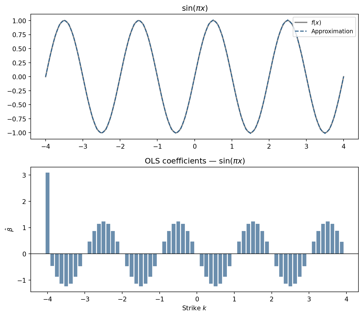
64 option-style basis functions are enough to closely track a function with four full oscillations. The options transform has a clear interpretation: the coefficients must oscillate in sign to produce the alternating peaks and troughs of the sine. Each \(\hat\beta_j\) says how much slope to add at strike \(k_j\); alternating positive and negative contributions generate the up-down rhythm of the wave.
\(\text{sinc}(x)\)
The sinc function \(\text{sinc}(x) = \sin(\pi x) / (\pi x)\) is smooth but its oscillations decay away from the origin. The options transform must reflect that concentration.
fig, axes = plt.subplots(2, 1, figsize=(8, 7))
x, knots, beta, y_hat = fit(np.sinc, -6, 6)
plot_fit(axes[0], axes[1], x, knots, beta, y_hat, np.sinc, r"$\mathrm{sinc}(x)$")
fig.tight_layout(); plt.show()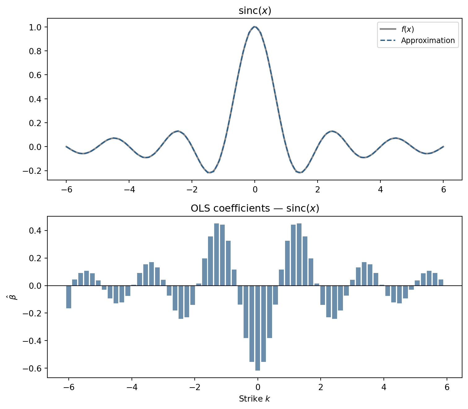
The coefficients are large near the origin and taper toward the edges, mirroring the function’s own shape.
Heaviside \(H(x)\)
The Heaviside function is the opposite challenge: piecewise constant with a single discontinuity. The basis must spend its degrees of freedom precisely at \(x = 0\).
fig, axes = plt.subplots(2, 1, figsize=(8, 7))
x, knots, beta, y_hat = fit(lambda x: np.heaviside(x, 0.5), -2, 2)
plot_fit(axes[0], axes[1], x, knots, beta, y_hat, lambda x: np.heaviside(x, 0.5), r"Heaviside $H(x)$")
fig.tight_layout(); plt.show()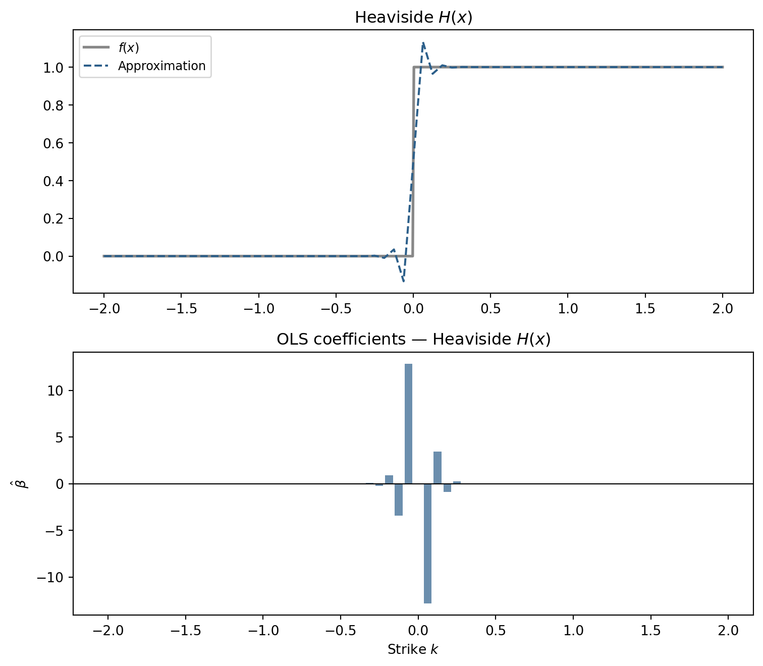
The coefficients spike near \(x = 0\) and are nearly zero elsewhere. The OLS procedure discovers the discontinuity by loading all the adjustment at the one point where slope needs to change abruptly. The approximation cannot perfectly reproduce the jump—these are piecewise-linear functions—but it localizes the transition sharply.
The Deeper Connection
What makes this assignment worthwhile is not the coding—the Python is simple. The interesting part is that the same exercise connects three ideas that are usually presented in separate courses:
- Ross (1976): A rich enough set of option payoffs can span any contingent claim. The coefficients here are a finite-dimensional version of that spanning argument.
- Breeden and Litzenberger (1978): In the continuum limit, the second derivative of an option price with respect to strike recovers the risk-neutral density. Our \(\hat\beta\) vector is a discrete analogue: differences in adjacent coefficients reveal the “weight” placed on each region of the domain.
- Universal approximation (Bengio et al. 2017): The theoretical result that single-hidden-layer networks with ReLU activations can approximate any continuous function on a compact set is exactly the statement that the basis \(\{h(x - k_j)\}\) is rich enough—provided \(n\) is large enough.
Ross, Stephen A. 1976. “Options and Efficiency.” Quarterly Journal of Economics 90 (1): 75–89.
Breeden, Douglas T., and Robert H. Litzenberger. 1978. “Prices of State-Contingent Claims Implicit in Option Prices.” Journal of Business 51 (4): 621–51. https://doi.org/10.1086/296025.
Bengio, Yoshua, Ian Goodfellow, and Aaron Courville. 2017. Deep Learning. MIT press Cambridge, MA, USA.
The hidden layer of a neural network, from this angle, is not a mysterious black box. It is a portfolio of option-style payoffs, and training the network is the problem of finding the right portfolio weights.