Modeling Stock Prices in Continuous-Time

Options, Futures and Derivative Securities

Lorenzo Naranjo

Spring 2026

From Binomial Trees to Brownian Motion

The Log Price in a Binomial Tree

• With u = e^{\sigma \sqrt{\Delta t}} and d = e^{-\sigma \sqrt{\Delta t}}, each period adds \sigma \sqrt{\Delta t} to \ln(S) or subtracts it.
• After m periods, at time t = m \Delta t, \ln(S_{t}) = \ln(S_{0}) + \sigma \sqrt{\Delta t} \, (X_{1} + X_{2} + \cdots + X_{m}), where X_{i} = +1 for an up move and -1 for a down move.
• With independent, equally likely moves, \operatorname{V}\left(\ln(S_{t})\right) = \sigma^{2} \Delta t \times m = \sigma^{2} t.
• The variance grows in proportion to time, however short the periods.
  • Steps proportional to \Delta t would give variance \sigma^{2} t \Delta t \to 0: the price would stop moving.
  • Steps that do not shrink would make the variance explode.

The Scaled Random Walk

• Setting \sigma aside, the random part of the log price is the scaled random walk B_{t}^{(n)} = \sqrt{\Delta t} \, (X_{1} + X_{2} + \cdots + X_{m}), \qquad t = m \Delta t, with n = 1 / \Delta t steps per unit of time.
• Its mean is zero and its variance is m \Delta t = t, for every n.

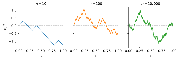
One path of the scaled random walk over 0 \leq t \leq 1 with n = 10, n = 100, and n = 10{,}000 steps per unit of time.

Brownian Motion

• As \Delta t \to 0, B_{t}^{(n)} is a sum of more and more independent, ever smaller steps.
• By the central limit theorem, its distribution approaches \mathcal{N}(0, t).
• The same holds for the change over any interval (s, t], which is independent of the steps taken before.
• The limit is called a Brownian motion, or a Wiener process.

Brownian Motion

A Brownian motion \{B_{t} \colon t \geq 0\} is a stochastic process such that:

1. B_{0} = 0.
2. For s < t, the increment B_{t} - B_{s} is normally distributed with mean zero and variance t - s.
3. Increments over non-overlapping intervals are independent.
4. The path t \mapsto B_{t} is continuous.

Brownian Motion Simulation

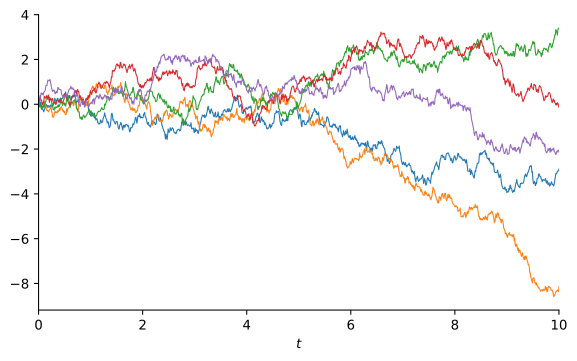
Simulated paths of a Brownian motion \left\{B_{t}\right\} for t \in [0, 10].

Properties of Brownian Motion

• B_{t} \sim \mathcal{N}(0, t), so B_{t} = \sqrt{t} \, Z for a standard normal Z.
• The increments are normal because of the central limit theorem, not because the coin flips were normal.
  • Any steps with mean zero and variance one lead to the same limit.
• The paths are continuous but nowhere smooth.
  • Over an interval of length dt, the increment dB has standard deviation \sqrt{dt}, much larger than dt.
  • A Brownian path moves a lot over every short interval.
• This single fact is why calculus with Brownian motion differs from ordinary calculus.

Geometric Brownian Motion

Geometric Brownian Motion

• A Brownian motion is not a good model for the price itself.
  • It can become negative.
  • Its changes do not depend on its level, while a $200 stock moves about twice as many dollars as at $100.
• What is roughly stable over time is the distribution of returns: \frac{\Delta S_{t}}{S_{t}} = \mu \Delta t + \sigma \Delta B_{t} \sim \mathcal{N}(\mu \Delta t, \sigma^{2} \Delta t).
• Letting \Delta t \to 0 gives the geometric Brownian motion (GBM) dS = \mu S \, dt + \sigma S \, dB.
• \mu is the expected return and \sigma the volatility, the same \sigma used to build binomial trees.

GBM Simulation

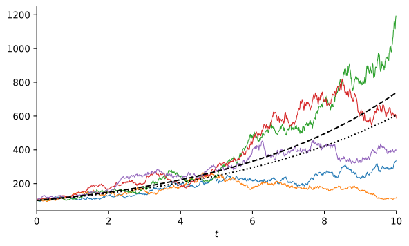
Simulated paths of a GBM with S_{0} = 100, \mu = 0.20, and \sigma = 0.20. The dashed line is \mathbb{E}\left( S_{t} \right) = S_{0} e^{\mu t} and the dotted line is the median S_{0} e^{(\mu - \frac{1}{2} \sigma^{2}) t}.

• Paths stay positive, fluctuate more at higher prices, and fan out unevenly.

Itô’s Lemma

Why Ordinary Calculus Fails

• In ordinary calculus, \Delta F \approx F'(x) \, \Delta x + \frac{1}{2} F''(x) (\Delta x)^{2}, and the second-order term is negligible because (\Delta x)^{2} is tiny compared with \Delta x.
• For a Brownian motion, \Delta B is of order \sqrt{\Delta t}, so (\Delta B)^{2} is of order \Delta t.
• The second-order term no longer disappears.

Squared Increments Add Up to Time

• (\Delta B)^{2} = \Delta t \, Z^{2} has mean \Delta t and variance 2 (\Delta t)^{2}: a single one is far from \Delta t.
• Split [0, t] into n steps of length \Delta t = t/n and add up the squared increments: \operatorname{E}\left(\textstyle\sum (\Delta B)^{2}\right) = n \Delta t = t, \qquad \operatorname{V}\left(\textstyle\sum (\Delta B)^{2}\right) = n \times 2 (\Delta t)^{2} = 2 t \, \Delta t \to 0.

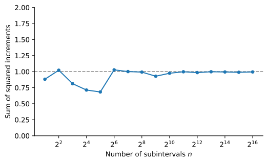
Sum of squared increments of one Brownian path on [0, 1] with n = 2, 4, \ldots, 2^{16} subintervals.

The Multiplication Table

• In differential notation, (dB)^{2} = dt: squared increments add up like increments of time.
• (dt)^{2} and (dt)(dB) are of order (dt)^{2} and (dt)^{3/2}, and they add up to zero.

Multiplication Table

(dB)^{2} = dt, \qquad (dt)(dB) = 0, \qquad (dt)^{2} = 0.

• For a GBM, (dS)^{2} = (\mu S \, dt + \sigma S \, dB)^{2} = \sigma^{2} S^{2} \, dt.
• The drift does not contribute to (dS)^{2}; only the random term does.

Itô’s Lemma

Itô’s Lemma

Let dS = \mu S \, dt + \sigma S \, dB and let F(S, t) be twice differentiable in S and differentiable in t. Then dF = \frac{\partial F}{\partial S} \, dS + \frac{1}{2} \frac{\partial^{2} F}{\partial S^{2}} \, (dS)^{2} + \frac{\partial F}{\partial t} \, dt, where (dS)^{2} = \sigma^{2} S^{2} \, dt. Substituting dS, dF = \left(\mu S \frac{\partial F}{\partial S} + \frac{1}{2} \sigma^{2} S^{2} \frac{\partial^{2} F}{\partial S^{2}} + \frac{\partial F}{\partial t}\right) dt + \sigma S \frac{\partial F}{\partial S} \, dB.

• It is a second-order Taylor expansion that keeps (dS)^{2}; the multiplication table kills every other second-order term.

Reading Itô’s Lemma

• \frac{1}{2} \sigma^{2} S^{2} \frac{\partial^{2} F}{\partial S^{2}} is the Itô correction.
  • It has no counterpart in ordinary calculus.
  • It vanishes when \sigma = 0 or when F is linear in S.
• When F depends only on S, the \partial F / \partial t term drops out.
• F is driven by the same Brownian motion as the stock, with random term \sigma S \frac{\partial F}{\partial S} \, dB.
  • This common source of risk is what allows an option to be replicated with the stock in the Black-Scholes model.

Example 1: Discounted Stock Price

• Let F(S, t) = e^{-r t} S, the stock price discounted at the risk-free rate r.
• Then \frac{\partial F}{\partial S} = e^{-r t}, \frac{\partial^{2} F}{\partial S^{2}} = 0, and \frac{\partial F}{\partial t} = -r e^{-r t} S, so dF = \left(\mu e^{-r t} S - r e^{-r t} S\right) dt + \sigma e^{-r t} S \, dB = (\mu - r) F \, dt + \sigma F \, dB.
• The discounted stock price is a GBM with expected return \mu - r, the risk premium, and the same volatility.
• There is no Itô correction because F is linear in S.

The Distribution of the Stock Price

Solving for the Stock Price

• Apply Itô’s lemma to F(S) = \ln(S), with \frac{\partial F}{\partial S} = 1/S and \frac{\partial^{2} F}{\partial S^{2}} = -1/S^{2}: d\ln(S) = \frac{1}{S} \, dS - \frac{1}{2} \frac{1}{S^{2}} \sigma^{2} S^{2} \, dt = \left(\mu - \tfrac{1}{2} \sigma^{2}\right) dt + \sigma \, dB.
• The coefficients are constant, so the changes add up to \ln(S_{T}) - \ln(S_{0}) = \left(\mu - \tfrac{1}{2} \sigma^{2}\right) T + \sigma B_{T} \quad \Longrightarrow \quad S_{T} = S_{0} e^{\left(\mu - \frac{1}{2} \sigma^{2}\right) T + \sigma B_{T}}.
• The log price is a Brownian motion with drift \mu - \frac{1}{2} \sigma^{2}: the continuous-time version of the log price in a binomial tree.
• -\frac{1}{2} \sigma^{2} is the Itô correction; ordinary calculus would give a log price growing at the rate \mu.

The Lognormal Distribution

• Since B_{T} \sim \mathcal{N}(0, T), \ln(S_{T}) \sim \mathcal{N}(m, s^{2}), \qquad m = \ln(S_{0}) + \left(\mu - \tfrac{1}{2} \sigma^{2}\right) T, \qquad s = \sigma \sqrt{T}.
• S_{T} has a lognormal distribution.
• The continuously compounded return \ln(S_{T} / S_{0}) is normal with mean \left(\mu - \frac{1}{2} \sigma^{2}\right) T and standard deviation \sigma \sqrt{T}.
• Probabilities about the stock price are computed by translating them into statements about this normal return.

Example 2: Probability Interval

• A stock follows a GBM with \mu = 12\%, \sigma = 25\%, and S_{0} = \$25.
• Over T = 0.5 years, X_{T} = \ln(S_{T}) has \begin{aligned} \operatorname{E}(X_{T}) & = \ln(25) + \left(0.12 - 0.5 (0.25)^{2}\right)(0.5) = 3.2633, \\ \operatorname{SD}(X_{T}) & = 0.25 \sqrt{0.5} = 0.1768. \end{aligned}
• Exponentiating the endpoints of 3.2633 \pm 1.96 (0.1768), \left[e^{3.2633 - 1.96 (0.1768)}, e^{3.2633 + 1.96 (0.1768)}\right] = [18.48, 36.96].
• There is a 95% probability that the price in six months lies between $18.48 and $36.96.
• The interval is not symmetric around $25: the lognormal distribution is skewed to the right.

Moments of the Stock Price

Moments of the Stock Price

If dS = \mu S \, dt + \sigma S \, dB, then \operatorname{E}(S_{T}) = S_{0} e^{\mu T}, \qquad \operatorname{SD}(S_{T}) = \operatorname{E}(S_{T}) \sqrt{e^{\sigma^{2} T} - 1}.

• They follow from the lognormal moments: \operatorname{E}(S_{T}) = e^{m + \frac{1}{2} s^{2}} = S_{0} e^{\mu T}.
• The expected price grows at the rate \mu, which is why \mu is called the expected return.
• The standard deviation grows even faster than the expected price.

Example 3

• For the stock in Example 2, the expected price and standard deviation six months from now are \operatorname{E}(S_{T}) = 25 e^{0.12 (0.5)} = \$26.55, \qquad \operatorname{SD}(S_{T}) = 26.55 \sqrt{e^{0.25^{2} (0.5)} - 1} = \$4.73.

Expected Return and Growth Rate

• The log price grows at the rate \mu - \frac{1}{2} \sigma^{2}; the expected price grows at the faster rate \mu.
• The gap comes from the skewness of the lognormal distribution: \text{Median}(S_{T}) = S_{0} e^{\left(\mu - \frac{1}{2} \sigma^{2}\right) T} < S_{0} e^{\mu T} = \operatorname{E}(S_{T}).
• Half of the paths end below the median, and more than half end below the mean.
  • A few paths that end very high pull the mean above what a typical path achieves.
• \mu - \frac{1}{2} \sigma^{2} is the growth rate a long-term holder typically realizes; \mu is the rate at which wealth grows on average across paths.

Example 4: Growth Rate

• A stock has \mu = 0.10 and \sigma = 0.20, so its log price grows at 0.10 - 0.5 (0.20)^{2} = 0.08 per year.
• Over T = 10 years:
  • The expected price is e^{0.10 \times 10} = 2.72 times the current price.
  • The median price is only e^{0.08 \times 10} = 2.23 times the current price.
• The stock ends below its expected price when \sigma B_{T} < \frac{1}{2} \sigma^{2} T, which has probability \operatorname{P}\left(Z < \tfrac{1}{2} \sigma \sqrt{T}\right) = \operatorname{Φ}(0.3162) = 0.6241.

Looking Ahead

• The Black-Scholes model prices options with this lognormal distribution, with one change: the expected return \mu is replaced by the risk-free rate r.
• The Black-Scholes Model explains why.