Calibrating the Heston Model to AAPL Options
I just finished a new notebook on calibrating the Heston model and wanted to share it here. It works through the full pipeline: implementing the pricing formula in Python, loading real AAPL option data, and fitting the model parameters to the observed prices.
One thing I have noticed is that practical examples of using Heston are surprisingly rare. Most treatments stop at the derivation and leave the reader to figure out implementation on their own. Part of the reason is that Heston is not plug-and-play the way Black-Scholes is. With Black-Scholes you can back out implied volatility directly from a single option price. With Heston, the parameters \((\kappa, \theta, \sigma, \rho)\) have no direct market observable — you have to calibrate them jointly to a cross-section of prices. That extra step is a real barrier, and I think it explains why many people learn the model in theory but never get it running on real data.
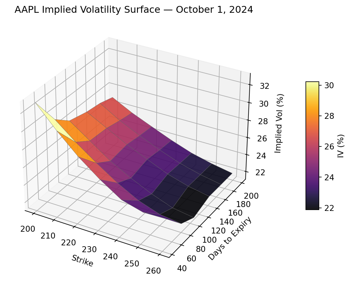
The surface below shows exactly what the model needs to match: implied volatilities are highest for low strikes and decay as the strike rises, with a steeper skew at short maturities that flattens as expiry moves further out. Fitting this structure with just four parameters is what calibration is all about.
The model
The Heston model is one of the workhorses of quantitative finance. It extends Black-Scholes by letting volatility itself follow a stochastic process. The stock price and its instantaneous variance evolve jointly as
\[ \begin{aligned} dS &= (r - q)\, S\, dt + \sqrt{v}\, S\, dB^S, \\ dv &= \kappa(\theta - v)\, dt + \sigma \sqrt{v}\, dB^v, \end{aligned} \]
where \(dB^S\) and \(dB^v\) are correlated Brownian motions with \(dB^S dB^v = \rho\, dt\). The variance \(v\) mean-reverts to its long-run level \(\theta\) at speed \(\kappa\), and \(\sigma\) controls how much \(v\) itself fluctuates. The correlation \(\rho\) links stock returns to volatility moves, producing the leverage effect observed in equity markets.
What makes Heston tractable is that despite this richer structure, the call price takes a form that closely mirrors Black-Scholes:
\[ C = S e^{-q T} P_1 - K e^{-r T} P_2. \]
The familiar Black-Scholes formula has the same structure, with \(N(d_1)\) and \(N(d_2)\) in place of \(P_1\) and \(P_2\). In Heston, \(P_2\) is the risk-neutral probability of expiring in the money and \(P_1\) is the corresponding probability under the stock-numeraire measure. Both are recovered by Fourier inversion of the model’s characteristic function rather than from a closed-form normal CDF, but the economic interpretation is identical. The complexity is hidden inside those two probabilities; the pricing formula itself stays clean.
What calibration means
Heston generates the implied volatility skew that equity options actually exhibit, which Black-Scholes cannot. But that extra realism comes at a cost: none of the parameters \((\kappa, \theta, \sigma, \rho)\) can be read directly off the market. Calibration is the step that bridges theory and data — given a cross-section of observed option prices, find the parameter vector that makes the model agree with the market.
Calibration is an inverse problem. The Heston pricing formula takes five parameters \((v_0, \kappa, \theta, \sigma, \rho)\) as inputs and returns a call price. Calibration runs this in reverse: given observed prices \(C^{\text{obs}}(K_i, T_j)\) across \(m\) strikes and \(n\) maturities, find the parameters that minimize the root mean-squared pricing error
\[ \text{RMSE} = \sqrt{\frac{1}{mn} \sum_{i=1}^{m} \sum_{j=1}^{n} \left(C^{\text{obs}}(K_i, T_j) - C^{\text{model}}(K_i, T_j)\right)^2}. \]
The notebook calibrates four parameters \((\kappa, \theta, \sigma, \rho)\) to 42 contracts spanning seven strikes and six maturities from 45 to 198 days, using AAPL call prices from October 1, 2024.
Fixing \(v_0\)
Treating \(v_0\) as a free parameter creates a degeneracy. A large \(\kappa\) paired with a \(v_0\) far from the short-term implied variance can produce nearly identical prices as a moderate \(\kappa\) with a well-anchored \(v_0\); the two parameters compensate each other and the optimizer wanders. Fixing \(v_0\) breaks the degeneracy, reduces the problem from five free parameters to four, and ties the short end of the volatility surface to a directly observable quantity.
The natural choice is to set \(v_0\) equal to the squared Black-Scholes implied volatility of the nearest-ATM option in the shortest maturity. This means the model matches that single contract exactly by construction, and the optimizer is free to fit the remaining structure.
What the parameters say
Once calibrated, each parameter has a clean economic interpretation.
The speed of mean reversion \(\kappa\) controls how quickly instantaneous variance returns to its long-run level \(\theta\). As \(\kappa \to \infty\) the variance process becomes nearly deterministic and the model collapses toward a constant-volatility world. The long-run variance \(\theta\) sets the volatility level that long-dated at-the-money options are priced against; its square root \(\sqrt{\theta}\) is directly comparable to long-dated implied volatility.
The volatility of volatility \(\sigma\) governs the curvature of the surface. A larger \(\sigma\) produces a more pronounced smile because the variance process itself is more uncertain. The correlation \(\rho\) captures the leverage effect: negative values make price drops and variance increases co-move, tilting the surface into the downward-sloping skew that is characteristic of equity markets.
Parameter estimates
The table below shows the calibrated parameter estimates.
| Description | Estimate | √ | |
|---|---|---|---|
| Parameter | |||
| v₀ | Initial variance (fixed) | 0.0709 | 0.2662 |
| κ | Speed of mean reversion | 3.4879 | — |
| θ | Long-run variance | 0.0627 | 0.2504 |
| σ | Vol of vol | 0.8174 | — |
| ρ | Correlation | -0.4823 | — |
Pricing errors
The overall RMSE across all 42 contracts is 0.2070 dollars. The table below breaks this down into mean absolute errors by strike and expiry, with row and column averages on the margins.
| Nov-24 | Dec-24 | Jan-25 | Feb-25 | Mar-25 | Apr-25 | Avg | |
|---|---|---|---|---|---|---|---|
| Strike | |||||||
| 200 | 0.462000 | 0.145000 | 0.066000 | 0.059000 | 0.000000 | 0.082000 | 0.136 |
| 210 | 0.542000 | 0.110000 | 0.125000 | 0.002000 | 0.055000 | 0.103000 | 0.156 |
| 220 | 0.576000 | 0.092000 | 0.235000 | 0.027000 | 0.017000 | 0.043000 | 0.165 |
| 230 | 0.549000 | 0.046000 | 0.240000 | 0.097000 | 0.018000 | 0.023000 | 0.162 |
| 240 | 0.378000 | 0.018000 | 0.252000 | 0.066000 | 0.037000 | 0.009000 | 0.127 |
| 250 | 0.249000 | 0.051000 | 0.274000 | 0.067000 | 0.069000 | 0.056000 | 0.128 |
| 260 | 0.153000 | 0.041000 | 0.209000 | 0.053000 | 0.073000 | 0.078000 | 0.101 |
| Avg | 0.415384 | 0.071775 | 0.200037 | 0.053076 | 0.038411 | 0.055978 | 0.139 |
Where the model falls short
The largest errors occur in short-maturity contracts. This is a structural limitation of Heston: the model-implied skew is proportional to \(\sqrt{T}\) as maturity shrinks, so it flattens too quickly near expiry and cannot match the steep short-dated skew that equity markets actually display. Multifactor extensions that allow the variance process to have richer dynamics can substantially improve the fit, as shown in Cortazar et al. (2017) in the context of commodity markets.
Despite this, the model reproduces the main features of the surface — the level, the skew, and the term structure of volatility — with just four free parameters, which makes it a natural starting point for any stochastic volatility application.