import os
import platform
from pathlib import Path

import matplotlib as mpl
import matplotlib.pyplot as plt
import numpy as np
import pandas as pd
import psycopg
from psycopg.types.numeric import FloatLoader
from scipy.optimize import minimize
from scipy.special import gammainc, gammaincc, gammaln

# Make SVG figures byte-identical across reruns, so the frozen outputs
# change in git only when a figure does
os.environ.setdefault("SOURCE_DATE_EPOCH", "0")
mpl.rcParams["svg.hashsalt"] = "waiting-for-the-nth-trade"

DATA_DIR = Path("../_data")


def wrds_username():
    """The WRDS username, read from the pgpass file."""
    if platform.system() == "Windows":
        pgpass = Path(os.environ["APPDATA"]) / "postgresql" / "pgpass.conf"
    else:
        pgpass = Path.home() / ".pgpass"
    for line in pgpass.read_text().splitlines():
        if line.startswith("wrds-pgdata"):
            return line.split(":")[3]


def load_wrds(name, sql):
    """Run a query on WRDS and cache the result in DATA_DIR/<name>.parquet."""
    file = DATA_DIR / f"{name}.parquet"
    if not file.exists():
        with psycopg.connect(host="wrds-pgdata.wharton.upenn.edu", port=9737,
                             dbname="wrds", user=wrds_username(),
                             sslmode="require") as conn:
            # Return SQL numbers as floats rather than Python Decimals
            conn.adapters.register_loader("numeric", FloatLoader)
            cur = conn.execute(sql)
            df = pd.DataFrame(cur.fetchall(), columns=[c.name for c in cur.description])
        DATA_DIR.mkdir(exist_ok=True)
        df.to_parquet(file)
return pd.read_parquet(file)Waiting for the n-th Trade
Introduction
If trades in a bond arrive as a Poisson process with rate \lambda, the times between trades are independent exponential random variables, and the waiting time W_n until the n-th trade, the sum of n of them, has a \text{Gamma}(n, \lambda) distribution. This notebook takes the gamma model to one day of corporate bond transactions from Enhanced TRACE. We keep \alpha and \lambda the same for every bond, but we estimate the shape \alpha instead of fixing it at n, so the estimate tells us how far the data are from the Poisson benchmark. We estimate the model for the first through the tenth trade, under three assumptions about when trades happen during the day. Under the Poisson model the estimated shapes line up with \alpha = n, and the rates are the same for every n.
The density of a \text{Gamma}(\alpha, \lambda) random variable is f(w) = \frac{\lambda^\alpha}{\Gamma(\alpha)} w^{\alpha - 1} e^{-\lambda w}, \qquad w > 0, \tag{1} with mean \operatorname{E}(W) = \alpha / \lambda and variance \alpha / \lambda^2.
Data
We use all trades executed on Wednesday, October 15, 2025. The sample consists of corporate bonds with at least one customer trade in the month before that day, which keeps out the thousands of bonds outstanding that almost never trade. Bonds in the sample that do not trade on October 15 stay in, because they tell us how long the wait can be.
day = load_wrds("trace_2025-10-15", """
    SELECT cusip_id, trd_exctn_tm, trc_st, msg_seq_nb, orig_msg_seq_nb,
           entrd_vol_qt, rptd_pr, rpt_side_cd, cntra_mp_id, sub_prdct, wis_fl
    FROM trace_enhanced.trace_enhanced
    WHERE trd_exctn_dt = '2025-10-15'
""")

universe = load_wrds("trace_universe_2025-10-15", """
    SELECT DISTINCT cusip_id
    FROM trace_enhanced.trace_enhanced
    WHERE trd_exctn_dt BETWEEN '2025-09-15' AND '2025-10-14'
      AND cntra_mp_id = 'C'
      AND trc_st = 'T'
      AND sub_prdct = 'CORP'
""")
TRACE records errors as separate rows that point back to the original trade report. We follow the filter of Dick-Nielsen (2014) for data reported after February 2012. A cancellation (X) or correction (C) repeats the original report with the same message sequence number, and both the original and the cancellation or correction are deleted. A correction also files a replacement report (R) with the correct terms, which stays in the data. A reversal (Y) points to the original through orig_msg_seq_nb, and both are deleted. Besides the sequence number, a report is matched to the original on CUSIP, volume, price, execution time, side and counterparty.
Dick-Nielsen, Jens. 2014. How to Clean Enhanced TRACE Data. Working Paper. Copenhagen Business School.
We then keep customer trades only (cntra_mp_id = 'C'). A trade between two dealers is reported by both, and a dealer who buys from a customer often sells to another dealer seconds later, so counting interdealer trades would produce many artificially short waits. Time is measured in hours from 8:00 a.m. Eastern, and the day ends at 5:00 p.m., nine hours later.
match = ["cusip_id", "entrd_vol_qt", "rptd_pr", "trd_exctn_tm", "rpt_side_cd",
         "cntra_mp_id", "msg_seq_nb"]
cancelled = day[day.trc_st.isin(["X", "C"])]
reversed_ = day[day.trc_st == "Y"].drop(columns="msg_seq_nb").rename(
    columns={"orig_msg_seq_nb": "msg_seq_nb"})
dead = pd.concat([cancelled[match], reversed_[match]]).drop_duplicates()

trades = day[day.trc_st.isin(["T", "R"])].merge(dead, on=match, how="left", indicator=True)
trades = trades[trades._merge == "left_only"].drop(columns="_merge")

trades = trades[
    (trades.cntra_mp_id == "C")
    & (trades.sub_prdct == "CORP")
    & (trades.wis_fl != "Y")
    & trades.cusip_id.isin(universe.cusip_id)
]

hours = pd.to_timedelta(trades.trd_exctn_tm.astype(str)).dt.total_seconds() / 3600 - 8
trades = trades.assign(t=hours)[(hours > 0) & (hours <= 9)]

counts = trades.groupby("cusip_id").size().reindex(universe.cusip_id, fill_value=0)
print(f"Bonds in the sample:          {len(counts):,}")
print(f"Customer trades on the day:   {counts.sum():,}")
print(f"Bonds with no trade:          {(counts == 0).mean():.1%}")
for k in [1, 2, 5, 10]:
    print(f"Bonds with {k:>2} or more:        {(counts >= k).mean():.1%}")
Bonds in the sample: 31,603
Customer trades on the day: 69,085
Bonds with no trade: 65.7%
Bonds with 1 or more: 34.3%
Bonds with 2 or more: 25.4%
Bonds with 5 or more: 12.8%
Bonds with 10 or more: 5.1%For each bond that trades at least n times, the waiting time w_{n,i} is the time of its n-th customer trade.
by_bond = trades.sort_values("t").groupby("cusip_id").t
n_bonds = len(counts)


def waits(n):
    """Time of the n-th customer trade of each bond that trades n times."""
    return by_bond.nth(n - 1).to_numpy()
Maximum likelihood with censoring
We observe each bond until some time T. A bond whose n-th trade happens at w_{n,i} \leq T contributes the density (1) to the likelihood. A bond that has not traded n times by T contributes the probability of that event, \operatorname{P}(W_n > T) = 1 - F(T). Writing n_c for the number of censored bonds, the log-likelihood is \ell(\alpha, \lambda) = \sum_{w_{n,i} \leq T} \Big( \alpha \ln \lambda - \ln \Gamma(\alpha) + (\alpha - 1) \ln w_{n,i} - \lambda w_{n,i} \Big) + n_c \ln Q(\alpha, \lambda T), \tag{2} where Q(\alpha, x) = \Gamma(\alpha, x) / \Gamma(\alpha) is the regularized upper incomplete gamma function, so that 1 - F(T) = Q(\alpha, \lambda T). Dropping the censored bonds would keep only the bonds that trade often and bias \lambda upward. Because every bond is observed over the same window, the censoring term is the only adjustment needed.
Later we let the rate change during the day. The code is written for that case from the start, using the expected number of trades by time t, \Lambda(t) = \int_0^t \lambda(s) \, ds, which equals \lambda t when the rate is constant. We take \lambda(t) to be constant between break points, so a single break at \tau gives \Lambda(t) = \lambda_1 \min(t, \tau) + \lambda_2 \max(t - \tau, 0). We maximize over \ln \alpha and the log rates to keep all parameters positive, and compute standard errors from a numerical Hessian of the log-likelihood.
def clock(t, rates, breaks):
    edges = np.concatenate([[0.0], breaks, [np.inf]])
    widths = np.diff(edges)
    return sum(r * np.clip(t - e, 0, d) for r, e, d in zip(rates, edges, widths))


def intensity(t, rates, breaks):
    return np.asarray(rates)[np.searchsorted(breaks, t)]


def neg_loglik(theta, w, T, breaks):
    alpha, rates = np.exp(theta[0]), np.exp(theta[1:])
    obs = w[w <= T]
    L = clock(obs, rates, breaks)
    observed = (alpha - 1) * np.log(L) - L - gammaln(alpha) + np.log(intensity(obs, rates, breaks))
    censored = (n_bonds - len(obs)) * np.log(gammaincc(alpha, clock(T, rates, breaks)))
    return -(observed.sum() + censored)


def hessian(f, x, h=1e-4):
    k = len(x)
    H = np.empty((k, k))
    E = h * np.eye(k)
    for i in range(k):
        for j in range(k):
            H[i, j] = (f(x + E[i] + E[j]) - f(x + E[i] - E[j])
                       - f(x - E[i] + E[j]) + f(x - E[i] - E[j])) / (4 * h**2)
    return H


def fit(w, T, breaks=(), alpha0=1.0):
    breaks = np.asarray(breaks, dtype=float)
    f = lambda theta: neg_loglik(theta, w, T, breaks)
    start = np.concatenate([[np.log(alpha0)], np.zeros(len(breaks) + 1)])
    res = minimize(f, start, method="Nelder-Mead",
                   options={"xatol": 1e-8, "fatol": 1e-8, "maxiter": 20000})
    se = np.sqrt(np.diag(np.linalg.inv(hessian(f, res.x))))
    lo, hi = np.exp(res.x[0] - 1.96 * se[0]), np.exp(res.x[0] + 1.96 * se[0])
    return {"alpha": np.exp(res.x[0]), "alpha 95% CI": f"[{lo:.2f}, {hi:.2f}]",
            "alpha lo": lo, "alpha hi": hi,
            "rates": np.exp(res.x[1:]), "breaks": breaks, "loglik": -res.fun}
The opening hours
Corporate bonds trade over the counter, so there is no opening bell, but almost no customer trades happen before 8:00 a.m. Eastern, an hour and a half before the stock market opens. We first fit the model to that window alone, so T = 1.5 and a bond is censored if it has not traded n times by 9:30. Here and below we start each search at the Poisson value \alpha = n.
ns = range(1, 11)


def fit_all(T, breaks=(), ns=ns):
    return {n: fit(waits(n), T, breaks, alpha0=n) for n in ns}


for n in ns:
    print(f"Bonds reaching trade {n:>2} by 9:30: {(waits(n) <= 1.5).sum():>5,}")
Bonds reaching trade 1 by 9:30: 2,243
Bonds reaching trade 2 by 9:30: 518
Bonds reaching trade 3 by 9:30: 148
Bonds reaching trade 4 by 9:30: 64
Bonds reaching trade 5 by 9:30: 31
Bonds reaching trade 6 by 9:30: 21
Bonds reaching trade 7 by 9:30: 12
Bonds reaching trade 8 by 9:30: 9
Bonds reaching trade 9 by 9:30: 6
Bonds reaching trade 10 by 9:30: 6Few bonds trade often enough before 9:30 to estimate the shape for large n: only 31 reach their fifth trade and 6 their tenth. We therefore fit the opening window for n \leq 4, where at least 64 bonds reach the n-th trade.
opening = fit_all(T=1.5, ns=range(1, 5))
for n, m in opening.items():
    print(f"n = {n}: alpha = {m['alpha']:.2f} {m['alpha 95% CI']}, lambda = {m['rates'][0]:.4f}")
n = 1: alpha = 0.99 [0.95, 1.03], lambda = 0.0475
n = 2: alpha = 1.66 [1.51, 1.82], lambda = 0.0741
n = 3: alpha = 2.47 [2.07, 2.94], lambda = 0.1282
n = 4: alpha = 2.64 [2.02, 3.44], lambda = 0.1112The wait for the first trade has \hat\alpha_1 = 0.99, the exponential distribution the Poisson model predicts. The estimates for the second and third trades, 1.66 and 2.47, fall short of n but not by much, and the fourth, 2.64, falls further short. Before the stock market opens, the first few bond trades arrive roughly the way the Poisson model describes.
The whole day
Extending the window to the close, T = 9, and keeping one rate for the whole day gives a very different shape.
constant = fit_all(T=9)
for n in ns:
    m = constant[n]
    print(f"n = {n:>2}: alpha = {m['alpha']:.2f} {m['alpha 95% CI']}, lambda = {m['rates'][0]:.4f}")
n = 1: alpha = 0.85 [0.83, 0.86], lambda = 0.0353
n = 2: alpha = 1.30 [1.26, 1.33], lambda = 0.0538
n = 3: alpha = 1.65 [1.60, 1.70], lambda = 0.0666
n = 4: alpha = 1.89 [1.83, 1.96], lambda = 0.0721
n = 5: alpha = 2.09 [2.02, 2.17], lambda = 0.0749
n = 6: alpha = 2.25 [2.16, 2.35], lambda = 0.0759
n = 7: alpha = 2.43 [2.32, 2.55], lambda = 0.0793
n = 8: alpha = 2.53 [2.41, 2.66], lambda = 0.0776
n = 9: alpha = 2.66 [2.52, 2.81], lambda = 0.0789
n = 10: alpha = 2.75 [2.59, 2.92], lambda = 0.0772Figure 1 compares the fitted distribution functions with the empirical ones for a few values of n. Since every bond is observed for the same nine hours, the empirical F(t) is simply the fraction of all bonds in the sample whose n-th trade came by time t.
grid = np.linspace(0, 9, 400)
hour_labels = [f"{h}:00" for h in range(8, 13)] + [f"{h}:00" for h in range(1, 6)]
shown = [1, 2, 5, 10]


def empirical_cdf(w):
    return np.searchsorted(np.sort(w), grid, side="right") / n_bonds


def fitted_cdf(model):
    return gammainc(model["alpha"], clock(grid, model["rates"], model["breaks"]))


def plot_fits(models):
    fig, ax = plt.subplots(figsize=(7, 4.5))
    for n, color in zip(shown, ["C0", "C1", "C2", "C3"]):
        ax.plot(grid, empirical_cdf(waits(n)), color=color, label=rf"$n = {n}$")
        ax.plot(grid, fitted_cdf(models[n]), color=color, linestyle="--")
    ax.set_xticks(range(10), hour_labels)
    ax.set_xlabel("Time of day (Eastern)")
    ax.set_ylabel(r"$P(W_n \leq t)$")
    ax.set_xlim(0, 9)
    ax.set_ylim(0)
    ax.legend(frameon=False)
    plt.tight_layout()
    plt.show()
plot_fits(constant)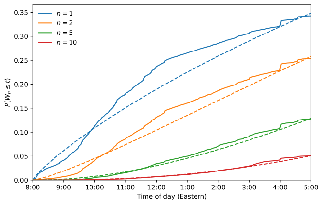
Over the whole day the estimates fall well below n, from 0.85 for the first trade to 2.75 for the tenth. In Figure 1 the fitted curves for the first and second trades rise too early and too slowly. The shape parameter governs how a curve starts, since F(t) \approx (\lambda t)^\alpha / \Gamma(\alpha + 1) for small t. A single rate has to match both the quiet opening and the busy late morning, and lowering \alpha is the only way the model can make the curve rise faster later in the day, at the cost of rising too fast at the start. The fifth and tenth trades come mostly after 9:30, and there the fitted curves follow the empirical ones closely.
A rate that changes at 9:30
The empirical curves bend when the stock market opens. The simplest way to capture this is to let the rate jump at \tau = 1.5, so that the bond market has one rate before 9:30 and another after. With the clock \Lambda(t) in place of \lambda t, the waiting time is still gamma distributed in the sense that \operatorname{P}(W_n \leq t) = P(\alpha, \Lambda(t)), where P = 1 - Q is the regularized lower incomplete gamma function. The model adds one parameter.
jump = fit_all(T=9, breaks=[1.5])
for n in ns:
    m = jump[n]
    print(f"n = {n:>2}: alpha = {m['alpha']:.2f} {m['alpha 95% CI']}, "
          f"rates = {m['rates'][0]:.4f}, {m['rates'][1]:.4f}, "
          f"ratio = {m['rates'][1] / m['rates'][0]:.1f}, "
          f"gain = {m['loglik'] - constant[n]['loglik']:.1f}")
n = 1: alpha = 0.58 [0.57, 0.60], rates = 0.0053, 0.0184, ratio = 3.5, gain = 335.6
n = 2: alpha = 0.79 [0.76, 0.81], rates = 0.0033, 0.0230, ratio = 7.0, gain = 440.8
n = 3: alpha = 1.03 [0.99, 1.06], rates = 0.0036, 0.0307, ratio = 8.5, gain = 291.2
n = 4: alpha = 1.23 [1.18, 1.28], rates = 0.0047, 0.0362, ratio = 7.8, gain = 170.8
n = 5: alpha = 1.41 [1.34, 1.47], rates = 0.0054, 0.0399, ratio = 7.4, gain = 108.6
n = 6: alpha = 1.57 [1.49, 1.66], rates = 0.0072, 0.0431, ratio = 5.9, gain = 66.8
n = 7: alpha = 1.74 [1.64, 1.85], rates = 0.0092, 0.0471, ratio = 5.1, gain = 41.7
n = 8: alpha = 1.87 [1.74, 2.01], rates = 0.0116, 0.0481, ratio = 4.1, gain = 26.0
n = 9: alpha = 2.01 [1.85, 2.19], rates = 0.0143, 0.0509, ratio = 3.6, gain = 16.5
n = 10: alpha = 2.15 [1.95, 2.37], rates = 0.0180, 0.0525, ratio = 2.9, gain = 10.2plot_fits(jump)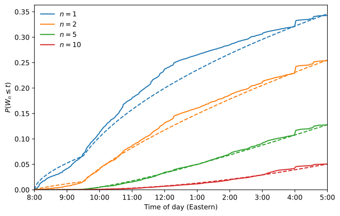
Figure 2 shows that the jump at 9:30 reproduces the bend in the curves for the first and second trades. The first trade is fitted worst: the model puts too many first trades before 9:30 and too few in the late morning. For one extra parameter, the log-likelihood rises by 336 for the first trade, 441 for the second and 291 for the third. The gain then shrinks steadily, to 10 for the tenth trade, which a single rate already fits well in Figure 1.
The rate after 9:30 is 3.5 times the rate before it for the first trade, 8.5 times for the third and 2.9 times for the tenth. Under a single Poisson process this ratio would be the same whichever trade we wait for. The levels of the rates cannot be compared across models or across n, because a different \alpha needs a different clock to produce the same curve; only their ratio is informative.
Comparing the models
Figure 3 collects the estimates of the shape from the three models, and Table 1 lists them with their confidence intervals. The fits for different n use the same bonds, and a bond’s tenth trade comes after its second, so the confidence intervals hold one at a time, not jointly.
models = {
    "Opening hours, 8:00 to 9:30": opening,
    "Whole day, constant rate": constant,
    "Whole day, rate jumps at 9:30": jump,
}
fig, ax = plt.subplots(figsize=(7, 4.5))
ax.plot([0.5, 10.5], [0.5, 10.5], color="gray", linestyle="--", label=r"Poisson, $\alpha = n$")
for (label, fits), shift, marker in zip(models.items(), [-0.15, 0, 0.15], ["s", "o", "^"]):
    x = np.array(list(fits)) + shift
    a = np.array([m["alpha"] for m in fits.values()])
    lo = np.array([m["alpha lo"] for m in fits.values()])
    hi = np.array([m["alpha hi"] for m in fits.values()])
    ax.errorbar(x, a, yerr=[a - lo, hi - a], fmt=marker, capsize=2, label=label)
ax.set_xticks(list(ns))
ax.set_xlim(0.5, 10.5)
ax.set_ylim(0)
ax.set_xlabel("Trade number $n$")
ax.set_ylabel(r"Shape $\alpha$")
ax.legend(frameon=False)
plt.tight_layout()
plt.show()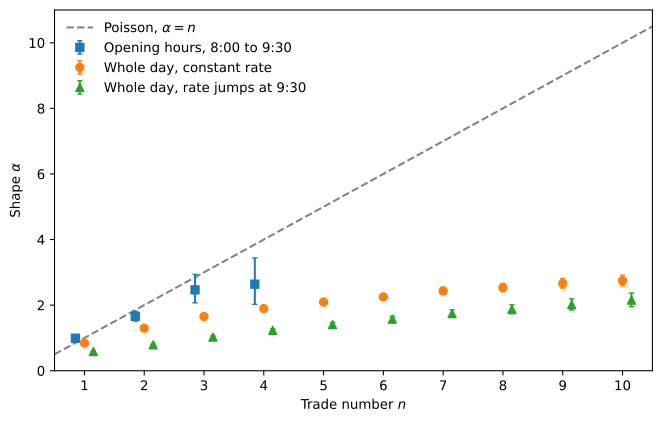
pd.DataFrame(
    {label: [f"{fits[n]['alpha']:.2f} {fits[n]['alpha 95% CI']}" if n in fits else ""
             for n in ns]
     for label, fits in models.items()},
    index=pd.Index(ns, name="n"),
)| Opening hours, 8:00 to 9:30 | Whole day, constant rate | Whole day, rate jumps at 9:30 | |
|---|---|---|---|
| n | |||
| 1 | 0.99 [0.95, 1.03] | 0.85 [0.83, 0.86] | 0.58 [0.57, 0.60] |
| 2 | 1.66 [1.51, 1.82] | 1.30 [1.26, 1.33] | 0.79 [0.76, 0.81] |
| 3 | 2.47 [2.07, 2.94] | 1.65 [1.60, 1.70] | 1.03 [0.99, 1.06] |
| 4 | 2.64 [2.02, 3.44] | 1.89 [1.83, 1.96] | 1.23 [1.18, 1.28] |
| 5 | 2.09 [2.02, 2.17] | 1.41 [1.34, 1.47] | |
| 6 | 2.25 [2.16, 2.35] | 1.57 [1.49, 1.66] | |
| 7 | 2.43 [2.32, 2.55] | 1.74 [1.64, 1.85] | |
| 8 | 2.53 [2.41, 2.66] | 1.87 [1.74, 2.01] | |
| 9 | 2.66 [2.52, 2.81] | 2.01 [1.85, 2.19] | |
| 10 | 2.75 [2.59, 2.92] | 2.15 [1.95, 2.37] |
Before the stock market opens, the estimates for the first three trades lie close to the Poisson line. Over the whole day they grow far more slowly than n: by about 0.2 per trade with a constant rate and 0.17 with the jump at 9:30. Removing the intraday pattern moves the estimates further from the Poisson line, not closer, since the jump model gives a lower \hat\alpha_n than the constant rate at every n.
What the estimates say
Once the intraday pattern is removed, the remaining departure from the Poisson model is a shape parameter that starts below 1 and grows far more slowly than n. That is what a mixture of slow and fast bonds produces: a mixture of gamma distributions with different rates has more mass at both short and long waits than any single member of the family. The counts point the same way. With a common rate, the number of trades a bond makes during the day would be Poisson, with variance equal to its mean.
print(f"Mean trades per bond: {counts.mean():.2f}")
print(f"Variance:             {counts.var():.2f}")
Mean trades per bond: 2.19
Variance: 194.31The variance is about ninety times the mean: a few bonds trade hundreds of times a day while most never trade. Some of the low \hat\alpha_n may also come from trades clustering in time within a bond, which the customer-trade filter weakens but does not remove. With one day of data and one rate for all bonds, the two explanations cannot be told apart.
A model that covers every n at once gives each bond its own rate, drawn from a gamma distribution across bonds. The number of trades by time t is then negative binomial rather than Poisson, so its variance can exceed its mean, and the waiting time to the n-th trade has a closed-form distribution with a single extra parameter, the shape of the distribution of rates. We leave that model for another notebook. A further step lets the rate depend on bond characteristics, \lambda_i(t) = \lambda(t) \exp(\mathbf{x}_i' \pmb{\beta}), with amount outstanding, age, maturity and rating in \mathbf{x}_i, and checks whether \hat\alpha_n moves back toward n once that heterogeneity is accounted for. Time variation within a bond, beyond the time of day, leads to the autoregressive conditional duration model of Engle and Russell (1998).
Engle, Robert F., and Jeffrey R. Russell. 1998. “Autoregressive Conditional Duration: A New Model for Irregularly Spaced Transaction Data.” Econometrica 66 (5): 1127–62.