From Regression to Neural Networks

A neural network is a regression with a more flexible shape. Like a linear regression, it predicts an outcome from some inputs by choosing parameters that make the prediction errors small on the data. Unlike a linear regression, it can bend to fit relations that are not straight lines. This chapter builds a network from the regression you already know, explains how its parameters are found, and then turns to the problem that dominates machine learning in finance: a flexible model fits the data it was trained on too well, and its performance on new data is what counts.

Regression as minimizing a loss

A linear regression predicts an outcome y_i from an input x_i with a straight line, \hat{y}_i = \beta_0 + \beta_1 x_i. Ordinary least squares chooses the intercept and slope that minimize the mean squared error, L(\beta_0, \beta_1) = \frac{1}{n} \sum_{i=1}^{n} \left( y_i - \beta_0 - \beta_1 x_i \right)^2. \tag{1} The function L is called the loss. For a straight line, calculus gives the minimizing \beta_0 and \beta_1 in closed form, which is the formula a statistics package uses. For the models in this chapter no such formula exists, and the loss has to be minimized numerically. Seeing linear regression as one case of “choose the parameters that minimize a loss” is the step that leads to everything else.

Gradient descent

The gradient of the loss, \nabla L, points in the direction in which the loss rises fastest. Gradient descent starts from a guess for the parameters \pmb{\theta} and repeatedly takes a small step in the opposite direction, \pmb{\theta}_{k+1} = \pmb{\theta}_{k} - \eta \, \nabla L(\pmb{\theta}_{k}), \tag{2} where \eta > 0 is the learning rate, the size of the step. Near a minimum the gradient is close to zero, so the steps shrink and the parameters settle.

Figure 1: Gradient descent on the loss of a regression slope. With a small learning rate the steps approach the minimum steadily; with a learning rate that is too large they overshoot and move away from it.

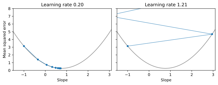
Figure 1 shows both behaviors for the slope of a simple regression. Choosing the learning rate is part of the work: too small and training takes forever, too large and it never settles. Modern variants of gradient descent, such as the Adam method used in the notebooks, adapt the step size as they go, but the idea is the same.

With millions of observations, computing the gradient on the whole sample at every step is slow. Stochastic gradient descent computes it on a small random batch of observations instead, which gives a noisy but cheap estimate. One pass through all the batches is called an epoch, and training usually runs for many epochs.

A neural network

A linear model can only draw straight lines (or flat planes, with several inputs). Many relations in finance are not straight. The payoff of a call option with strike K is \max(S - K, 0), flat below the strike and rising one-for-one above it, and an option’s price is a smooth curve with the same general shape.

A neural network with one hidden layer builds a curve out of simple pieces. Each of m hidden units computes a linear combination of the inputs \mathbf{x} and passes it through a nonlinear function g, and the output is a linear combination of the hidden units: \hat{y} = \beta_0 + \sum_{j=1}^{m} \beta_j \, g\left( w_{j0} + \mathbf{w}_j' \mathbf{x} \right). \tag{3} The function g is the activation. The most common choice today is the rectified linear unit, or ReLU, g(z) = \max(z, 0). A finance student has seen it before: it is the payoff of a call option. A network with ReLU activations is a weighted sum of call payoffs with different strikes and slopes, and sums of calls can approximate any reasonable payoff, which is why options can replicate so many payoffs and why networks can fit so many shapes.

Figure 2: A linear regression and a small neural network fitted to the same noisy data, generated from a call-option payoff. The network bends at the kink; the line cannot.

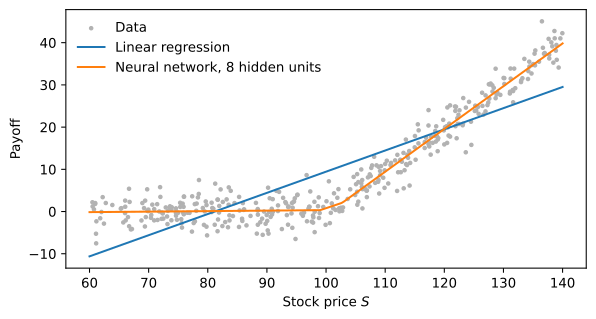
Figure 2 fits both models to data generated from a call payoff with strike 100 plus noise. The network has eight hidden units, so it has 8 \times 2 + 8 + 1 = 25 parameters, against two for the line. Networks with more hidden units, or several hidden layers stacked on top of each other, can represent more complicated shapes. Their parameters are found exactly as before: define the loss (1), and minimize it by gradient descent (2). The gradient of a network’s loss is computed with the chain rule, layer by layer from the output back to the inputs, an algorithm called backpropagation. Libraries such as PyTorch do this automatically. Goodfellow et al. (2016) is the standard reference for all of this.

Goodfellow, Ian, Yoshua Bengio, and Aaron Courville. 2016. Deep Learning. MIT Press. https://www.deeplearningbook.org.

Overfitting

Flexibility has a cost. A network with enough parameters can fit the noise in its training data as well as the relation behind it, and then it predicts new data badly. This is overfitting, and it is the central problem of machine learning.

The defense is to judge a model only on data it was not trained on. The usual practice splits the sample in three:

• a training set, used to fit the parameters;
• a validation set, used to choose among models and to decide when to stop training;
• a test set, used once, at the end, to report how well the chosen model does.

Figure 3: Training and validation loss of a large network trained on 60 noisy observations. The training loss keeps falling; the validation loss falls, then rises as the network starts to fit noise.

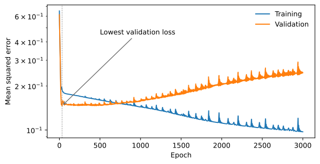
Figure 3 shows the typical pattern. Early in training, both losses fall: the network is learning the relation. Later, the training loss keeps falling while the validation loss rises: the network is memorizing the training noise. Stopping at the lowest validation loss, called early stopping, is one remedy. Others shrink the model’s flexibility directly, for example by penalizing large weights in the loss (weight decay) or by using fewer hidden units.

Why finance is hard for machine learning

The great successes of neural networks, in recognizing images or translating text, come from settings with enormous amounts of data and a strong signal: a photo of a cat is a cat. Asset returns are the opposite. Most of a stock’s monthly return is noise that no model can predict, so the signal is tiny compared with the noise, and the data are short, because there are only so many months.

Welch and Goyal (2008) show how hard this is even for linear models. They predict the stock market’s return with variables proposed in the literature, such as the dividend yield and interest rates, and find that out of sample these regressions do not beat the simplest forecast of all, the historical average return. A model can look good in the sample it was estimated on and lose to the average on new data.

Welch, Ivo, and Amit Goyal. 2008. “A Comprehensive Look at the Empirical Performance of Equity Premium Prediction.” Review of Financial Studies 21 (4): 1455–508.

Gu, Shihao, Bryan Kelly, and Dacheng Xiu. 2020. “Empirical Asset Pricing via Machine Learning.” Review of Financial Studies 33 (5): 2223–73. https://doi.org/10.1093/rfs/hhaa009.

Gu et al. (2020) find that machine learning does help, modestly. Forecasting the S&P 500 from forecasts of its individual stocks, a linear model has a monthly out-of-sample R^2 of -0.22\%, while trees and neural networks reach between 1.08\% and 1.80\%. They also find that network performance “peaks at three hidden layers then declines as more layers are added,” which they attribute to “the relatively small amount of data and tiny signal-to-noise ratio” of return prediction. In finance, a small model that predicts a little out of sample beats a large one that fits the past perfectly.

The out-of-sample R^2 used in these papers compares a model’s squared forecast errors with those of the historical average \bar{y}: R^2_{\text{OOS}} = 1 - \frac{\sum_{t} (y_t - \hat{y}_t)^2}{\sum_{t} (y_t - \bar{y}_t)^2}, \tag{4} where both forecasts use only data available before t. It is negative when the model does worse than the average, which happens often.

Practice Problems

These problems give you a chance to practice the concepts introduced in this chapter. Try to solve each one on your own before expanding the solution.

Problem 1 (Choosing a Learning Rate) You minimize a regression loss by gradient descent with three learning rates and record the loss after 50 steps:

Learning rate	Loss after 50 steps
0.001	0.912
0.1	0.251
2.0	4.7e12

Which statement is most accurate?

1. The learning rate of 0.001 is best, because small steps are always safer.
2. With a learning rate of 2.0 the steps overshoot the minimum and the loss explodes; 0.001 is too small to get close to the minimum in 50 steps; 0.1 works best here.
3. The learning rate does not matter, because gradient descent always finds the minimum.
4. A loss of 4.7e12 shows that the data contain errors.

Solution

The answer is (b). Each step moves the parameters by the learning rate times the gradient. When the rate is too large the step overshoots the minimum by more than it started away from it, so each step lands farther away and the loss grows without bound, as in the right panel of Figure 1. When it is too small the parameters move toward the minimum but slowly, so after 50 steps the loss is still high. A small rate is safe only in the sense that it does not explode, so (a) is wrong, and (c) and (d) ignore what the table shows.

Problem 2 (A Network Made of Call Payoffs) A network with one input S, two ReLU hidden units and no output intercept computes \hat{y} = 1 \times \max(S - 100, 0) - 1 \times \max(S - 110, 0). Compute \hat{y} for S = 90, S = 105 and S = 130, and name the option position whose payoff this network reproduces.

Solution

At S = 90 both terms are zero, so \hat{y} = 0. At S = 105 the first term is 5 and the second is zero, so \hat{y} = 5. At S = 130 the terms are 30 and 20, so \hat{y} = 10. The payoff is zero below 100, rises one-for-one between 100 and 110, and stays at 10 above 110. It is a bull call spread: long a call with strike 100 and short a call with strike 110. Each hidden unit is one call, and the output weights are the positions.

Problem 3 (A Model That Fits Well and Predicts Badly) You train a neural network to predict monthly market returns from ten predictors. On the training sample of 1950 to 2000 its R^2 is 35%. On 2001 to 2025, its out-of-sample R^2 relative to the historical average, as in (4), is -4\%. Select all statements that apply.

1. On 2001 to 2025, the network’s squared forecast errors are larger than those of the historical average return.
2. The high training R^2 shows the network has found a strong relation that will appear in future data.
3. The gap between the two numbers is a sign of overfitting.
4. A negative out-of-sample R^2 is impossible, so the calculation must be wrong.

Solution

The answers are (a) and (c). By (4), a negative out-of-sample R^2 means the model’s sum of squared errors exceeds that of the historical average, so (a) holds and (d) is wrong: unlike the in-sample R^2 of a regression with an intercept, the out-of-sample version has no lower bound of zero. A flexible model that explains 35% of returns in sample and loses to the average out of sample has fit noise in the training data, which is overfitting, so (c) holds and (b) does not.