Beta Pricing with Frontier Portfolios
Introduction
In the previous notebook we characterized the minimum-variance frontier (MVF) for an economy with n risky assets. We found that the set of frontier portfolios forms a hyperbola in the (\sigma, \mu) space and that any two frontier portfolios span the entire frontier. In this notebook we exploit the spanning property to establish a fundamental pricing result: the expected return of any asset is determined solely by how much it co-moves with any given frontier portfolio.
The key insight is that every asset can be decomposed into a frontier component and an idiosyncratic residual. The residual, by construction, has zero covariance with all frontier portfolios and therefore carries no compensation in expected returns — it is unpriced risk. What matters for pricing is only the systematic exposure to the frontier.
We develop this idea in three steps. First, we define the idiosyncratic risk of an asset and show it is uncorrelated with every frontier portfolio. Second, we establish that for every frontier portfolio p (other than the minimum variance portfolio) there exists a unique zero-covariance frontier portfolio z. Third, we combine these results to derive the beta-pricing formula \operatorname{E}(r_{i}) = \mu_{z} + \beta_{i}(\operatorname{E}(r_{p}) - \mu_{z}), where \beta_{i} = \operatorname{Cov}(r_{i}, r_{p}) / \sigma^{2}(r_{p}) and \mu_{z} is the expected return of the zero-covariance portfolio of p. The next notebook shows how this formula simplifies when a risk-free asset is present.1
1 Beta pricing needs only the law of one price, which makes portfolio returns weighted averages of asset returns (Definition 1 of the previous notebook). It does not need the absence of arbitrage, and it does not imply it. Beta pricing with respect to p says that a stochastic discount factor linear in r_{p}, m = a - b\,r_{p}, prices every asset. When r_{p} is unbounded above, m is negative in some states. That is harmless for the n assets, but extending m to payoffs outside their span can assign a negative price to a nonnegative payoff. Dybvig and Ingersoll (1982) show that if mean-variance pricing holds for all assets in a complete market and the market return can be high enough, a call option on the market with a high strike has a negative price, an arbitrage. Beta pricing can therefore price options without creating arbitrage only when its stochastic discount factor is strictly positive.
Beta Pricing
Property 1 (Idiosyncratic Risk) Consider an asset whose expected return is \mu_{i}. We define the idiosyncratic risk of the asset as the difference between its return, and the return of a frontier portfolio that has the same expected return. It turns out that the idiosyncratic risk of any asset is uncorrelated with all frontier portfolios.
Consider an arbitrary frontier portfolio with expected return \mu_{p} and pick any asset or portfolio with expected return \mu_{i}. The covariance between r_{p} and r_{i} is \begin{aligned} \operatorname{Cov}(r_{i}, r_{p}) & = \mathbf{w}_{i}' \mathbf{V} \mathbf{w}_{p} = \mathbf{w}_{i}' \mathbf{V} (\mathbf{a} + \mu_{p}\mathbf{b}) = \mathbf{w}_{i}' \left[\frac{1}{D}(B\pmb{\iota} - A\mathbf{e}) + \frac{\mu_{p}}{D}(C\mathbf{e} - A\pmb{\iota}) \right] \\ & = \dfrac{1}{D}\left(B - A\mu_{p} - A\mu_{i} + C\mu_{i}\mu_{p}\right). \end{aligned} This shows that two assets with the same expected return will have the same covariance with a given frontier portfolio p. This seemingly marginal property is at the heart of modern asset pricing. Given a frontier portfolio, what determines the expected return of any asset is how much it covaries with the frontier portfolio regardless of its total risk.
To look at this result in more detail, consider the frontier portfolio r_{p, i} with the same expected return as asset i. Define the residual \varepsilon_{i} = r_{i} - r_{p, i}. \tag{1} By construction, the residual has zero mean \operatorname{E}(\varepsilon_{i}) = \operatorname{E}(r_{i}) - \operatorname{E}(r_{p, i}) = 0, and if we pick any frontier portfolio p we also have that \operatorname{Cov}(r_{p}, \varepsilon_{i}) = \operatorname{Cov}(r_{p}, r_{i}) - \operatorname{Cov}(r_{p}, r_{p, i}) = 0. That is, the residual is unrelated to the returns of frontier portfolios. Since we just saw that the expected return of an asset depends only on how it covaries with a frontier portfolio, the residual is not priced, hence the name idiosyncratic risk.
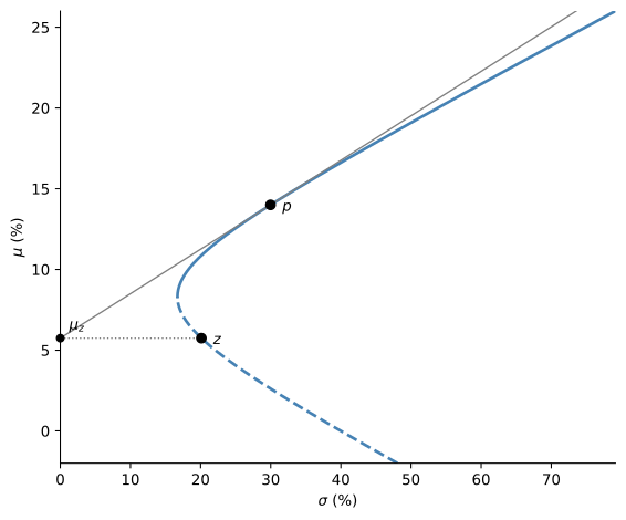
Property 2 (Zero-Covariance) For a given frontier portfolio p with expected return \mu_{p} and variance \sigma_{p}^2, we can always find (except for the minimum variance portfolio) a unique frontier portfolio z with expected return \mu_{z} that is uncorrelated with p, i.e. \operatorname{Cov}(r_{z}, r_{p}) = 0. Just draw a line that is tangent to the minimum-variance frontier at the point (\sigma_{p}, \mu_{p}). The intercept of this line with the vertical axis gives \mu_{z}.
Using the variance expression \sigma^{2} = (B - 2A\mu + C\mu^{2})/D, we can compute the derivative of \sigma with respect to \mu, \dfrac{d \sigma}{d \mu} = \dfrac{d \sqrt{\sigma^{2}}}{d \mu} = \dfrac{1}{2 \sigma} \dfrac{d \sigma^{2}}{d \mu} = \dfrac{C\mu - A}{D\sigma}. \tag{2} Denote by m_{p} the slope coefficient of the minimum variance frontier at the point (\sigma_{p}, \mu_{p}). Equation (2) implies that \frac{\sigma_{p}}{m_{p}} = \frac{C\mu_{p} - A}{D}, since d \sigma / d \mu = 1 / (d \mu / d \sigma) = 1 / m.
The equation of the tangent line to the minimum variance frontier at point (\sigma_{p}, \mu_{p}) is given by \mu - \mu_{p} = m_{p} (\sigma - \sigma_{p}). Denote by \mu_{z} the intercept of this line with the vertical axis. Then we have that \mu_{z} = \mu_{p} - m_{p} \sigma_{p}. We can now compute the covariance of r_{p} and a frontier portfolio r_{z} with expected return \mu_{z}. \begin{aligned} \operatorname{Cov}(r_{z}, r_{p}) & = \dfrac{1}{D}\left(B - A\mu_{p} - A\mu_{z} + C\mu_{z}\mu_{p}\right) \\ & = \dfrac{1}{D}\left(B - 2A\mu_{p} + C\mu_{p}^{2}\right) - \dfrac{\mu_{p} - \mu_{z}}{D}(C\mu_{p} - A) \\ & = \sigma_{p}^{2} - m_{p}\sigma_{p}\left(\frac{C\mu_{p} - A}{D}\right) = \sigma_{p}^{2} - m_{p}\sigma_{p}\left(\frac{\sigma_{p}}{m_{p}}\right) = 0. \end{aligned} Obviously, the covariance of the minimum variance portfolio with any other frontier portfolio is equal to its variance, so it is impossible to find a frontier portfolio that has zero-covariance with it.2
2 Geometrically, the tangent to the frontier at the minimum variance portfolio is vertical in (\sigma, \mu) space, so it has no finite intercept with the \mu-axis.
Figure 1 shows the construction for the frontier portfolio p with \mu_{p} = 14\%. The tangent at p meets the vertical axis at \mu_{z} \approx 5.7\%, and the zero-covariance portfolio z is the frontier portfolio with that mean. Because p is on the efficient branch, \mu_{z} is below the mean of the MVP and z lies on the inefficient branch.
Property 3 (Beta Pricing with Frontier Portfolios) Frontier portfolios contain all the information we need to price assets and carry all the systematic risk of the economy. Just pick any frontier portfolio p with return r_{p}, and compute its associated zero-covariance portfolio r_{z}. Then for any asset or portfolio i we have that r_{i} = (1 - \beta_{i}) r_{z} + \beta_{i} r_{p} + \varepsilon_{i}, where \beta_{i} = \dfrac{\operatorname{Cov}(r_{i}, r_{p})}{\sigma^{2}(r_{p})}, \qquad \operatorname{E}(\varepsilon_{i}) = \operatorname{Cov}(r_{p}, r_{z}) = \operatorname{Cov}(r_{p}, \varepsilon_{i}) = \operatorname{Cov}(r_{z}, \varepsilon_{i}) = 0.
Let \mu_{i} = \operatorname{E}(r_{i}). We start by re-writing (1) as r_{i} = r_{p, i} + \varepsilon_{i}, and note that r_{p, i} is a frontier portfolio, and hence it can be represented as a portfolio of any two other frontier portfolios. Therefore, just pick an arbitrary frontier portfolio p (but different from the minimum variance portfolio)3 with expected return \mu_{p}, and find its associated zero-covariance frontier portfolio z. We then form a portfolio composed of both frontier portfolios such that r_{p, i} = (1 - \beta_{i}) r_{z} + \beta_{i} r_{p}, with \beta_{i} = \frac{\mu_{i} - \mu_{z}}{\mu_{p} - \mu_{z}}. The choice for \beta_{i} guarantees that \operatorname{E}(r_{p, i}) = \mu_{i}. Note that \varepsilon_{i} is uncorrelated with both r_{z} and r_{p}, and that r_{z} and r_{p} are also uncorrelated. Hence, the covariance of r_{i} and r_{p} is given by \begin{aligned} \operatorname{Cov}(r_{i}, r_{p}) & = \operatorname{Cov}((1 - \beta_{i}) r_{z} + \beta_{i} r_{p} + \varepsilon_{i}, r_{p}) \\ & = (1 - \beta_{i}) \underbrace{\operatorname{Cov}(r_{z}, r_{p})}_{0} + \beta_{i} \underbrace{\operatorname{Cov}(r_{p}, r_{p})}_{\sigma^{2}(r_{p})} + \underbrace{\operatorname{Cov}(\varepsilon_{i}, r_{p})}_{0} = \beta_{i} \sigma^{2}(r_{p}), \end{aligned} which yields that \beta_{i} = \dfrac{\operatorname{Cov}(r_{i}, r_{p})}{\sigma^{2}(r_{p})}.
3 The restriction is necessary because, by Property 2, the zero-covariance portfolio z does not exist for the minimum variance portfolio.
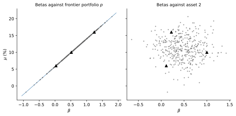
The result holds only because p is a frontier portfolio. Figure 2 computes betas for the three assets and for simulated portfolios of them against two benchmarks. Against the frontier portfolio p of Figure 1, every point lies exactly on the line through (0, \mu_{z}) and (1, \mu_{p}). Against asset 2, which lies inside the frontier, the same portfolios scatter and no line prices them. A linear relation between expected returns and betas therefore says only that the benchmark is a frontier portfolio, a point that returns in Roll’s critique of the CAPM.