Mean-Variance Analysis with N Risky Assets

Introduction

This notebook develops the mathematics of portfolio choice for an economy with n risky assets and no risk-free asset. The analysis follows Chapter 3 in Huang and Litzenberger (1988).

Huang, Chi-fu, and Robert H Litzenberger. 1988. Foundations for Financial Economics. North-Holland.

Markowitz, Harry. 1952. “The Utility of Wealth.” Journal of Political Economy 60 (2): 151–58.

Markowitz (1952) was the first to establish a solid foundation for this problem. His key insight is that combining risky assets allows investors to diversify away idiosyncratic risk, but some risk—known as systematic risk—cannot be eliminated. As a result, for any target expected return there is a portfolio that achieves the lowest possible variance, and the collection of all such portfolios traces out the minimum variance frontier (MVF).

Without short-selling constraints, the MVF is a hyperbola in (\mu, \sigma) space. We derive its equation explicitly, show that any two frontier portfolios span the entire frontier, and characterize the global minimum variance portfolio (MVP). Beta pricing and the extension to economies with a risk-free asset are covered in separate notebooks.

N-Risky Assets

Portfolio Statistics

We use lowercase boldface for vectors and uppercase boldface for matrices; \mathbf{A}' denotes the transpose of \mathbf{A}. The n asset returns and portfolio weights are collected in column vectors \mathbf{r} = (r_{1}, r_{2}, \ldots, r_{n})', \qquad \mathbf{w} = (w_{1}, w_{2}, \ldots, w_{n})'.

Investors allocate wealth across the n assets by choosing weights \mathbf{w}. Weights may be positive (long) or negative (short), subject only to the budget constraint \mathbf{w}'\pmb{\iota} = 1, where \pmb{\iota} = (1, 1, \ldots, 1)'. The portfolio return is therefore r = \mathbf{w}' \mathbf{r}. \tag{1}

For portfolio optimization we need the first two moments of \mathbf{r}. The vector of expected returns is \mathbf{e} = (\operatorname{E}(r_{1}), \operatorname{E}(r_{2}), \ldots, \operatorname{E}(r_{n}))', where \operatorname{E}(\cdot) denotes the expectation operator. The covariance matrix \mathbf{V}, with (i,j) entry \operatorname{Cov}(r_{i}, r_{j}), is symmetric by definition and positive semidefinite since for any \mathbf{y} \in \mathbb{R}^{n}, \mathbf{y}' \mathbf{V} \mathbf{y} = \mathbf{y}' \operatorname{E}\left[ (\mathbf{r} - \mathbf{e})(\mathbf{r} - \mathbf{e})' \right] \mathbf{y} = \operatorname{E}\left[ \left((\mathbf{r} - \mathbf{e})' \mathbf{y}\right)^{2} \right] \geq 0.

Definition 1 (Economy) An economy consists of n risky assets. Each asset i has a payoff x_i, a strictly positive price p_i > 0, and a net return r_i = x_i/p_i - 1. Prices satisfy the law of one price, so the price of a portfolio is the sum of the prices of its holdings. The vector \mathbf{r} = (r_1, \ldots, r_n)' has an invertible covariance matrix \mathbf{V}. The return of any portfolio is r = \mathbf{w}' \mathbf{r}.

For the returns \mathbf{r} to be well-defined, each price p_{i} must be strictly positive, and we assume this directly. The law of one price is what makes the return of a portfolio the weighted average \mathbf{w}'\mathbf{r} of the returns of its holdings. Nothing more is required of prices in these notebooks. In particular, we do not assume the absence of arbitrage, under which every nonnegative payoff has a nonnegative price. Like Chamberlain and Rothschild (1983), who take the cost of each asset as given and rule out only riskless profits, mean-variance analysis works with returns and their first two moments. The beta pricing notebook explains why this matters.

Chamberlain, Gary, and Michael Rothschild. 1983. “Arbitrage, Factor Structure, and Mean-Variance Analysis on Large Asset Markets.” Econometrica 51 (5): 1281–304.

We will assume that \mathbf{V} is invertible to guarantee that the n-risky basis assets are linearly independent, i.e. that no combination of them generates a risk-free asset. Intuitively, this implies that it is not possible to combine the risky assets to build a portfolio that has zero variance.

Since \mathbf{V} is symmetric, all its eigenvalues are real. Being positive semidefinite further requires all eigenvalues to be non-negative, while being invertible rules out zero eigenvalues. Together, these three properties imply that all eigenvalues of \mathbf{V} are strictly positive, so \mathbf{V} is positive definite: \mathbf{y}' \mathbf{V} \mathbf{y} > 0 for all \mathbf{y} \neq \mathbf{0}.

Property 1 (Portfolio Statistics) For portfolios of risky assets we have the following relations \operatorname{E}(r_{p}) = \mathbf{w}_{p}' \mathbf{e}, \qquad \sigma^{2}(r_{p}) = \mathbf{w}_{p}' \mathbf{V} \mathbf{w}_{p}, \qquad \operatorname{Cov}(r_{p}, r_{q}) = \mathbf{w}_{q}' \mathbf{V} \mathbf{w}_{p}.

Taking expectations in (1), the expected return of portfolio p is computed as \operatorname{E}(r_{p}) = \sum_{i = 1}^{n} w_{i, p} \operatorname{E}(r_{i}) = \mathbf{w}_{p}' \mathbf{e}. Applying (1) to portfolios p and q, the covariance between these two portfolios is \operatorname{Cov}(r_{p}, r_{q}) = \sum_{i = 1}^{n} \sum_{j = 1}^{n} w_{i, p} w_{j, q} \operatorname{Cov}(r_{i}, r_{j}) = \mathbf{w}_{q}' \mathbf{V} \mathbf{w}_{p} Finally, the variance of portfolio p is just \sigma^{2}(r_{p}) = \operatorname{Cov}(r_{p}, r_{p}) = \mathbf{w}_{p}' \mathbf{V} \mathbf{w}_{p}

The Minimum-Variance Frontier

Property 2 (The Minimum Variance Frontier) The minimum variance frontier contains all the portfolios that achieve the minimum possible variance for a given expected return. It determines the frontier of the investment opportunity set. It is an hyperbola characterized in (\mu, \sigma) space by \frac{\sigma^{2}}{1/C} - \frac{(\mu - A/C)^{2}}{D/C^{2}} = 1.

We want to solve the following problem: \min_{\mathbf{w}} \ \dfrac{1}{2} \mathbf{w}' \mathbf{V} \mathbf{w} \quad \textrm{s.t.} \quad \mathbf{w}' \mathbf{e} = \mu, \quad \mathbf{w}' \pmb{\iota} = 1.

For this we form the Lagrangian \mathcal{L} = \dfrac{1}{2} \mathbf{w}' \mathbf{V} \mathbf{w} + \lambda_{1} (\mu - \mathbf{w}' \mathbf{e}) + \lambda_{2} (1 - \mathbf{w}' \pmb{\iota})

The first order conditions for this problem are \dfrac{\partial \mathcal{L}}{\partial \mathbf{w}} = \mathbf{V} \mathbf{w} - \lambda_{1} \mathbf{e} - \lambda_{2} \pmb{\iota} = 0, \qquad \dfrac{\partial \mathcal{L}}{\partial \lambda_{1}} = \mu - \mathbf{w}' \mathbf{e} = 0, \qquad \dfrac{\partial \mathcal{L}}{\partial \lambda_{2}} = 1 - \mathbf{w}' \pmb{\iota} = 0. \tag{2} From the first FOC in (2), the frontier weights must lie in the span of \mathbf{V}^{-1}\mathbf{e} and \mathbf{V}^{-1}\pmb{\iota}: \mathbf{w} = \lambda_{1}\mathbf{V}^{-1}\mathbf{e} + \lambda_{2}\mathbf{V}^{-1}\pmb{\iota}. \tag{3}

Define A = \pmb{\iota}' \mathbf{V}^{-1} \mathbf{e}, \qquad B = \mathbf{e}' \mathbf{V}^{-1} \mathbf{e}, \qquad C = \pmb{\iota}' \mathbf{V}^{-1} \pmb{\iota}, and let D = BC - A^{2}. Substituting (3) into the two constraints gives B\lambda_{1} + A\lambda_{2} = \mu, \qquad A\lambda_{1} + C\lambda_{2} = 1. Solving, \lambda_{1} = \frac{C\mu - A}{D}, \qquad \lambda_{2} = \frac{B - A\mu}{D}. Therefore the frontier portfolio is affine in its target mean: \mathbf{w} = \mathbf{a} + \mu \mathbf{b}, where \mathbf{a} = \frac{1}{D}\mathbf{V}^{-1}(B\pmb{\iota} - A\mathbf{e}), \qquad \mathbf{b} = \frac{1}{D}\mathbf{V}^{-1}(C\mathbf{e} - A\pmb{\iota}). \tag{4} Hence, \sigma^{2} = (\mathbf{a} + \mu \mathbf{b})' \mathbf{V} (\mathbf{a} + \mu \mathbf{b}) = \dfrac{1}{D} (B - 2 A \mu + C \mu^{2}). \tag{5} This can be written as \frac{\sigma^{2}}{1/C} - \frac{(\mu - A/C)^{2}}{D/C^{2}} = 1. \tag{6} Equation (6) describes an hyperbola in (\mu, \sigma) space with vertex \left( 1/\sqrt{C}, A/C \right) and asymptotes \mu = A/C \pm \sigma \sqrt{D/C}.

Figure 1: Minimum variance frontier for three risky assets. Gray dots are simulated portfolios obtained by perturbing the equally weighted portfolio with a random shock that sums to zero across assets. The upper branch is the efficient frontier and the dashed lines are the asymptotes.

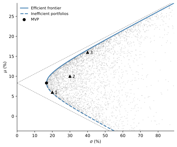
The investment opportunity set is the region on and to the right of the hyperbola in Figure 1, which the simulated portfolios fill. They crowd near the frontier because moving away from it at a fixed mean raises the variance quadratically, so interior points require larger long and short positions. To see this, write any portfolio with mean \mu as \mathbf{w} = \mathbf{w}_{p} + \mathbf{z}, where \mathbf{w}_{p} is the frontier portfolio with the same mean and \mathbf{z} satisfies \mathbf{z}'\mathbf{e} = \mathbf{z}'\pmb{\iota} = 0. Then \sigma^{2} = \mathbf{w}_{p}'\mathbf{V}\mathbf{w}_{p} + 2\mathbf{w}_{p}'\mathbf{V}\mathbf{z} + \mathbf{z}'\mathbf{V}\mathbf{z}. The cross term vanishes because, by (3), \mathbf{V}\mathbf{w}_{p} = \lambda_{1}\mathbf{e} + \lambda_{2}\pmb{\iota} for some scalars \lambda_{1},\lambda_{2}. Hence \mathbf{w}_{p}'\mathbf{V}\mathbf{z} = \lambda_{1}\mathbf{e}'\mathbf{z} + \lambda_{2}\pmb{\iota}'\mathbf{z} = 0. Since \mathbf{V} is positive definite, \mathbf{z}'\mathbf{V}\mathbf{z} \geq 0, and therefore \sigma^{2} \geq \sigma^{2}_{\min}(\mu) for every portfolio with mean \mu.

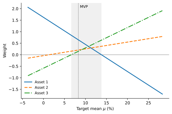
Figure 2 plots the three weights of (4) as the target mean varies. Each weight is a straight line in \mu, and the three lines add up to one at every target. In this example all three weights are positive only for targets between about 6.6% and 13.8%, an interval that contains the MVP. Below it the frontier portfolio shorts asset 3, the asset with the highest mean, and above it the portfolio shorts asset 1, the one with the lowest mean. Reaching extreme targets on the frontier therefore requires large long and short positions.

Figure 2: Frontier weights \mathbf{w} = \mathbf{a} + \mu\mathbf{b} as functions of the target mean \mu. The dotted line marks the MVP and the shaded band the targets for which all weights are positive.

Property 3 (Spanning) The investment opportunity set has dimension n and is spanned by n risky assets such that their covariance matrix is invertible. The minimum variance frontier has dimension 2 and is spanned by any two different frontier portfolios.

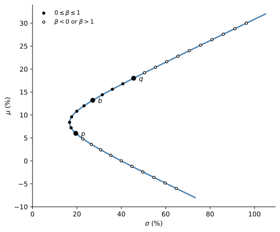
Consider two frontier portfolios, p and q with expected returns \mu_{p} and \mu_{q}. By (4), their weights are \mathbf{w}_{p} = \mathbf{a} + \mu_{p}\mathbf{b}, \qquad \mathbf{w}_{q} = \mathbf{a} + \mu_{q}\mathbf{b}. Consider now forming a portfolio b consisting of 1 - \beta of p and \beta of q. Its expected return is \mu_{b} = (1 - \beta) \mu_{p} + \beta \mu_{q}, and its portfolio weights are given by \mathbf{w}_{b} = (1 - \beta)(\mathbf{a} + \mu_{p}\mathbf{b}) + \beta(\mathbf{a} + \mu_{q}\mathbf{b}) = \mathbf{a} + \left[(1 - \beta)\mu_{p} + \beta\mu_{q}\right]\mathbf{b} = \mathbf{a} + \mu_{b}\mathbf{b}, which shows that b is also a frontier portfolio. Letting \beta range over all real numbers, including values outside [0, 1] that short one of the two portfolios, traces out the entire frontier. Figure 3 illustrates this for p and q, with b = 0.4\, p + 0.6\, q labeled.

Figure 3: Spanning: combinations (1 - \beta)\,p + \beta\,q of two frontier portfolios trace out the whole MVF. Filled dots have 0 \leq \beta \leq 1, open dots short one of the two portfolios, and b = 0.4\,p + 0.6\,q is labeled.

Property 4 (Minimum Variance Portfolio) There is a unique portfolio that minimizes variance across all portfolios, called the minimum variance portfolio (MVP), denoted by g. The covariance of the MVP with any other portfolio is always equal to the variance of the MVP.

We solve the problem: \min_{\mathbf{w}} \ \dfrac{1}{2} \mathbf{w}' \mathbf{V} \mathbf{w} \quad \textrm{s.t.} \quad \mathbf{w}' \pmb{\iota} = 1.

For this we form the Lagrangian \mathcal{L} = \dfrac{1}{2} \mathbf{w}' \mathbf{V} \mathbf{w} + \lambda (1 - \mathbf{w}' \pmb{\iota})

The first order conditions for this problem are \dfrac{\partial \mathcal{L}}{\partial \mathbf{w}} = \mathbf{V} \mathbf{w} - \lambda \pmb{\iota} = 0, \qquad \dfrac{\partial \mathcal{L}}{\partial \lambda} = 1 - \mathbf{w}' \pmb{\iota} = 0. Hence \mathbf{w}_{g} = \lambda \mathbf{V}^{-1} \pmb{\iota}, and the budget constraint pins down \lambda: 1 = \mathbf{w}_{g}' \pmb{\iota} = \lambda \pmb{\iota}' \mathbf{V}^{-1} \pmb{\iota} = \lambda C \qquad \Longrightarrow \qquad \mathbf{w}_{g} = \dfrac{1}{C} \mathbf{V}^{-1} \pmb{\iota}. The covariance of the MVP with any other portfolio i is given by \operatorname{Cov}(r_{i}, r_{g}) = \mathbf{w}_{i}' \mathbf{V} \mathbf{w}_{g} = \mathbf{w}_{i}' \mathbf{V} \left( \frac{1}{C} \mathbf{V}^{-1} \pmb{\iota} \right) = \frac{\mathbf{w}_{i}' \pmb{\iota}}{C} = \frac{1}{C}. Since \operatorname{V}(r_{g}) = \operatorname{Cov}(r_{g}, r_{g}) = 1 / C, we have that \operatorname{Cov}(r_{i}, r_{g}) = \operatorname{V}(r_{g}) for any portfolio i.

Note that the standard deviation of the MVP corresponds to the \sigma-coordinate of the vertex of the hyperbola described by (6).