Mean-Variance Analysis with a Risk-Free Asset
Introduction
In the previous notebook we derived the beta-pricing formula for economies with n risky assets. We showed that any frontier portfolio p and its zero-covariance counterpart z together price all assets: \operatorname{E}(r_i) = \mu_z + \beta_i(\operatorname{E}(r_p) - \mu_z). In this notebook we add a risk-free asset to the economy and show how the geometry and the pricing formula simplify considerably.
The key insight is that the risk-free asset is uncorrelated with every risky portfolio, so it naturally plays the role of the zero-covariance portfolio. The minimum-variance frontier, which was a hyperbola in the all-risky case, collapses to a pair of rays emanating from r_f on the \mu-axis. The upper ray is the efficient frontier, and the unique risky frontier portfolio where this ray touches the risky-asset frontier is the tangency portfolio.
We proceed in three steps. First, we characterize portfolio statistics with a risk-free asset and show that the minimum-variance frontier is a pair of rays, a cone, whose slope is the maximum Sharpe ratio of the economy. Second, we identify the tangency portfolio q as the unique risky portfolio on both frontiers. Third, we show that beta pricing reduces to \operatorname{E}(r_i) = r_f + \beta_i (\operatorname{E}(r_q) - r_f), where \beta_i = \operatorname{Cov}(r_i, r_q) / \sigma^2(r_q). This is the foundation of any beta pricing model: all expected returns are explained by a single beta with respect to q. The CAPM, developed in Part II, adds an equilibrium argument to identify q with the market portfolio.
N-Risky Assets and a Risk-Free Asset
Portfolio Statistics
In this section we add a risk-free asset denoted by r_{f} to the investment opportunity set. Investors can allocate \mathbf{w} to the risky assets and 1 - \mathbf{w}' \pmb{\iota} to the risk-free asset, so that the returns of any portfolio can be expressed as r = \sum_{i = 1}^{n} w_{i} r_{i} + \Big(1 - \sum_{i = 1}^{n} w_{i}\Big) r_{f} = \mathbf{w}' \mathbf{r} + (1 - \mathbf{w}' \pmb{\iota}) r_{f}.
Note that the weights of the risky assets do not need to sum up to one since any amount not invested in the risky assets can be invested in the risk-free asset.
Definition 1 (Economy) We consider an economy spanned by n-risky assets with returns \mathbf{r} and a risk-free asset r_{f}. The risk-asset returns are such that no linear combination among them can synthesize a risk-free asset, i.e. \mathbf{V}^{-1} exists.
The returns r of any portfolio can be expressed as r = \mathbf{w}' \mathbf{r} + (1 - \mathbf{w}' \pmb{\iota}) r_{f}.
The condition that \mathbf{V} is invertible guarantees that the n-risky assets are linearly independent, i.e. no combination of them generates a risk-free asset. However, there is now a risk-free asset to invest. If there is no risk-free asset and \mathbf{V} is not invertible, it means that we can synthesize the risk-free asset from the existing risky assets. In that case we can compute the implied risk-free rate, reduce the dimension of the risky assets by one, and proceed as if there is a risk-free asset.
Property 1 (Portfolio Statistics with a Risk-Free Asset) For portfolios of risky assets and a risk-free asset we have the following relations \operatorname{E}(r_{p}) = \mathbf{w}_{p}' \mathbf{e} + (1 - \mathbf{w}_{p}' \pmb{\iota}) r_{f}, \qquad \sigma_{p}^{2} = \mathbf{w}_{p}' \mathbf{V} \mathbf{w}_{p}, \qquad \operatorname{Cov}(r_{p}, r_{q}) = \mathbf{w}_{q}' \mathbf{V} \mathbf{w}_{p}.
The expected return of portfolio p is given by \operatorname{E}(r_{p}) = \sum_{i = 1}^{n} w_{i, p} \operatorname{E}(r_{i}) + (1 - \sum_{i = 1}^{n} w_{i, p}) r_{f} = \mathbf{w}_{p}' \mathbf{e} + (1 - \mathbf{w}_{p}' \pmb{\iota}) r_{f}. Because r_{f} is a constant, every term of the covariance between portfolio p and another portfolio q that involves the risk-free asset vanishes, leaving \operatorname{Cov}(r_{p}, r_{q}) = \sum_{i = 1}^{n} \sum_{j = 1}^{n} w_{i, p} w_{j, q} \operatorname{Cov}(r_{i}, r_{j}) = \mathbf{w}_{q}' \mathbf{V} \mathbf{w}_{p}. Hence, the variance of portfolio p is just \operatorname{Cov}(r_{p}, r_{p}) = \mathbf{w}_{p}' \mathbf{V} \mathbf{w}_{p}.
The Minimum-Variance Frontier
Property 2 (Minimum Variance Frontier with a Risk-Free Asset) The investment opportunity set with a risk-free asset is a cone whose frontier is given by \sigma = \dfrac{|\mu - r_{f}|}{\mathit{SR}} where \mathit{SR} denotes the maximum Sharpe ratio attainable in the economy.
By allocating \mathbf{w} to the risky assets, and whatever is left, which is given by 1 - \mathbf{w}' \pmb{\iota}, to the risk-free asset, we avoid one restriction. Hence, we want to solve the following problem: \min_{\mathbf{w}} \ \dfrac{1}{2} \mathbf{w}' \mathbf{V} \mathbf{w} \quad \textrm{s.t.} \quad \mathbf{w}' \mathbf{e} + (1 - \mathbf{w}' \pmb{\iota}) r_{f} = \mu.
To simplify notation, we define \pmb{\eta} = \mathbf{e} - \pmb{\iota} r_{f}, \qquad \mu^{e} = \mu - r_{f}. The Lagrangian in this case is \mathcal{L} = \dfrac{1}{2} \mathbf{w}' \mathbf{V} \mathbf{w} + \lambda (\mu^{e} - \mathbf{w}' \pmb{\eta}). The first order conditions for this problem are \dfrac{\partial \mathcal{L}}{\partial \mathbf{w}} = \mathbf{V} \mathbf{w} - \lambda \pmb{\eta} = 0, \qquad \dfrac{\partial \mathcal{L}}{\partial \lambda} = \mu^{e} - \mathbf{w}' \pmb{\eta} = 0. \tag{1} From (1) we get that \mathbf{w} = \lambda \mathbf{V}^{-1} \pmb{\eta}, so that \mathbf{w}' \pmb{\eta} = \lambda \pmb{\eta}' \mathbf{V}^{-1} \pmb{\eta} = \mu^{e}. We finally have that \mathbf{w} = \dfrac{\mathbf{V}^{-1} \pmb{\eta}}{\pmb{\eta}' \mathbf{V}^{-1} \pmb{\eta}} \mu^{e}. \tag{2} Using (2) in \sigma^{2} = \mathbf{w}' \mathbf{V} \mathbf{w} = \left(\dfrac{\mu^{e}}{\pmb{\eta}' \mathbf{V}^{-1} \pmb{\eta}}\right)^{2} \pmb{\eta}' \mathbf{V}^{-1} \mathbf{V} \mathbf{V}^{-1} \pmb{\eta} = \dfrac{\left(\mu^{e}\right)^{2}}{\pmb{\eta}' \mathbf{V}^{-1} \pmb{\eta}}, which implies that \sigma = \dfrac{|\mu - r_{f}|}{\sqrt{\pmb{\eta}' \mathbf{V}^{-1} \pmb{\eta}}}. \tag{3} We note that the maximum Sharpe-ratio that is possible in this economy is \mathit{SR} = \sqrt{\pmb{\eta}' \mathbf{V}^{-1} \pmb{\eta}}.
The Tangency Portfolio
When there is a risk-free asset, there is a unique frontier portfolio composed exclusively of risky assets that also lies on the frontier of the enlarged investment opportunity set. This portfolio is called the tangency portfolio.
This question is equivalent to asking: Can we find \mu such that nothing is invested in the risk-free asset? Or equivalently, can we find \mu such that everything is invested into risky assets? If so, is this \mu unique? We will call the tangency portfolio q.
Starting from (2) and our constraint that we want to invest everything into risky securities 1 = \mathbf{w}' \pmb{\iota} = \dfrac{\pmb{\eta}' \mathbf{V}^{-1} \pmb{\iota}}{\pmb{\eta}' \mathbf{V}^{-1} \pmb{\eta}} \mu^{e}. We can now solve for \mu^{e} and see that the solution exists and is unique. Using this result into (2) we find \mathbf{w}_{q} = \dfrac{\mathbf{V}^{-1} \pmb{\eta}}{\pmb{\eta}' \mathbf{V}^{-1} \pmb{\iota}}. \tag{4}
Figure 1 puts the pieces together. Mixing the risk-free asset with risky portfolios fills a cone with vertex at r_{f}, bounded by two rays of slope \pm\mathit{SR}. The upper ray touches the risky-asset frontier at q. Between r_{f} and q, efficient portfolios lend at the risk-free rate; beyond q, they borrow to hold more than 100% in q.
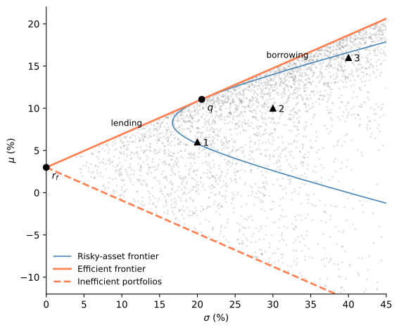
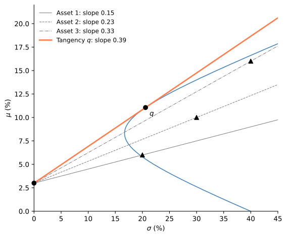
Figure 2 shows why the slope of the efficient frontier is the maximum Sharpe ratio. Every risky portfolio defines a ray from r_{f} whose slope is its Sharpe ratio, and mixing it with the risk-free asset moves along that ray. The individual assets have Sharpe ratios of 0.15, 0.23 and 0.33, and the steepest ray that still reaches a risky portfolio is the one tangent to the risky frontier, through q, with slope \mathit{SR} \approx 0.39.
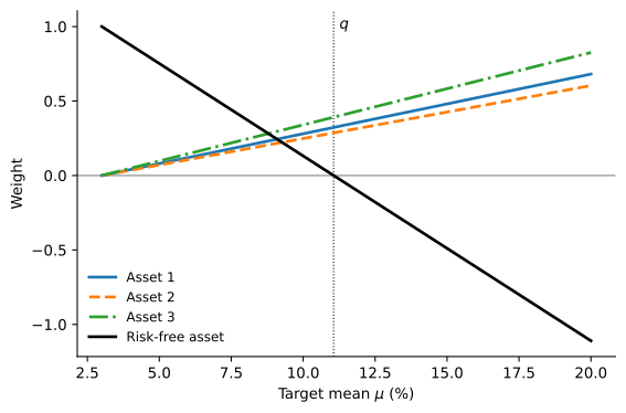
By (2), every efficient portfolio invests (\mu - r_{f})/(\mu_{q} - r_{f}) times \mathbf{w}_{q} in the risky assets and the rest in the risk-free asset. Figure 3 plots these weights as the target mean rises. The weight on each risky asset is a line through zero at r_{f}, and the three always stay in the proportions of q, about (0.32, 0.29, 0.39), while the risk-free weight falls from one and crosses zero at \mu_{q}. Only the split between q and the risk-free asset changes along the frontier. This is two-fund separation: every investor on the efficient frontier holds the same risky portfolio, in contrast with the all-risky case of the previous notebook, where the composition of frontier portfolios changes with the target.
Beta-Pricing
Beta-pricing simplifies considerably when a risk-free asset is available. Because r_f is a constant, it is uncorrelated with every risky portfolio and therefore serves as the zero-covariance portfolio for any frontier portfolio. In particular, for the tangency portfolio q and any asset or portfolio i we have r_{i} = (1 - \beta_{i}) r_{f} + \beta_{i} r_{q} + \varepsilon_{i} where \beta_{i} = \dfrac{\operatorname{Cov}(r_{i}, r_{q})}{\sigma^{2}(r_{q})}, \qquad \operatorname{E}(\varepsilon_{i}) = \operatorname{Cov}(r_{q}, \varepsilon_{i}) = 0. Taking expectations yields the beta-pricing formula (Roll 1977; Huang and Litzenberger 1988) \operatorname{E}(r_{i}) = r_{f} + \beta_{i} (\operatorname{E}(r_{q}) - r_{f}).
All systematic risk is captured by a single beta with respect to the tangency portfolio, and the risk-free rate replaces the zero-covariance return that appeared in the all-risky case. The CAPM notebook, at the start of Part II, adds an equilibrium argument (homogeneous beliefs and market clearing) to identify q with the market portfolio, yielding the Capital Asset Pricing Model (CAPM).