Class 6

Counting Events in Continuous Time

Defaults, insurance claims, order arrivals and price jumps happen at unpredictable moments. To model them, split [0, t] into n slots of length \Delta t = t / n and let an event occur in each slot with probability \lambda \Delta t, independently across slots. The count up to time t is binomial with mean \lambda t, and its PGF converges to a Poisson PGF, \left(1 + \frac{\lambda t (z - 1)}{n}\right)^{n} \xrightarrow[n \to \infty]{} e^{\lambda t (z - 1)}. Events in disjoint intervals come from disjoint slots, so they are independent. A Poisson process with rate \lambda > 0 is a process \{N_{t}\} with N_{0} = 0, independent increments, and N_{t} - N_{s} \sim \text{Poisson}(\lambda (t - s)) for s < t. Its paths are step functions that jump up by one at each event, and \operatorname{E}(N_{t}) = \operatorname{V}(N_{t}) = \lambda t, \qquad \operatorname{P}(\mathop{}\!\mathrm{d}N_{t} = 1) = \lambda \mathop{}\!\mathrm{d}t+ o(\mathop{}\!\mathrm{d}t), \qquad \operatorname{P}(\mathop{}\!\mathrm{d}N_{t} \geq 2) = o(\mathop{}\!\mathrm{d}t). \tag{1} Over a short interval there is either no event or a single one, with probability proportional to the length of the interval.

Superposition and Thinning

Independent Poisson processes with rates \lambda_{1} and \lambda_{2} add up to a Poisson process with rate \lambda_{1} + \lambda_{2}. Conversely, if each event is independently of type A with probability p, the type A and type B counts are independent Poisson processes with rates \lambda p and \lambda (1 - p). Many type A events signal a large total, which offsets the smaller share left for type B.

Waiting Times

The first event comes after t exactly when no event occurs in [0, t], so \operatorname{P}(T_{1} > t) = \operatorname{P}(N_{t} = 0) = e^{-\lambda t}, and the first waiting time is \text{Exp}(\lambda). The exponential distribution is memoryless, \operatorname{P}(T > s + t \mid T > s) = e^{-\lambda t} = \operatorname{P}(T > t), so time already spent waiting tells us nothing about the remaining wait. In credit risk, \lambda is the hazard rate: given survival to t, a firm defaults in (t, t + \mathop{}\!\mathrm{d}t] with probability \lambda \mathop{}\!\mathrm{d}t+ o(\mathop{}\!\mathrm{d}t). Memorylessness is what lets the process start afresh after each event: the times T_{1}, T_{2}, \ldots between consecutive events are iid \text{Exp}(\lambda), and conversely adding up iid exponential waiting times builds a Poisson process.

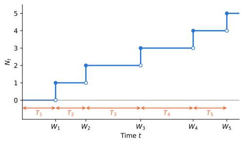
The time of the n-th event, W_{n} = T_{1} + \cdots + T_{n}, has a gamma distribution with mean n / \lambda and variance n / \lambda^{2}. Counts and arrival times describe the same paths, as Figure 1 shows, and \operatorname{P}(W_{n} \leq t) = \operatorname{P}(N_{t} \geq n) = 1 - \sum_{k = 0}^{n - 1} e^{-\lambda t} \frac{(\lambda t)^{k}}{k!}. \tag{2}

Figure 1: One simulated path of a Poisson process with rate \lambda = 1. The arrival times W_{n} are marked on the time axis, and the arrows below the path show the exponential interarrival times T_{n} = W_{n} - W_{n - 1}.

Martingales

Let \mathcal{F}_{t} be the information generated by the path up to time t. Increments are independent of \mathcal{F}_{s}, so conditional expectations of future increments are ordinary expectations. N_{t} only moves up, but removing its expected growth gives three martingales: M_{t} = N_{t} - \lambda t, \qquad M_{t}^{2} - \lambda t, \qquad Z_{t} = \exp\left(\theta N_{t} - \lambda t (e^{\theta} - 1)\right). \tag{3} They mirror S_{n}, S_{n}^{2} - n and e^{\theta S_{n} - n K(\theta)} for the random walk, with K the CGF of the steps X_{i}.

Compound Poisson Processes

When each event carries an iid size Y_{i}, independent of N_{t}, the process X_{t} = \sum_{i = 1}^{N_{t}} Y_{i} is a compound Poisson process. Conditioning on N_{t} gives \phi_{X_{t}}(u) = e^{\lambda t (\phi_{Y}(u) - 1)}, \qquad \operatorname{E}(X_{t}) = \lambda t \operatorname{E}(Y), \qquad \operatorname{V}(X_{t}) = \lambda t \operatorname{E}(Y^{2}), \tag{4} and M_{X_{t}}(\theta) = e^{\lambda t (M_{Y}(\theta) - 1)} when the MGF exists. The variance involves \operatorname{E}(Y^{2}) because both the number and the size of the jumps are random.

Credit Spreads

If a firm defaults at the first event of a Poisson process whose intensity \lambda is its hazard rate, the default time \tau is \text{Exp}(\lambda). A zero-coupon bond paying one dollar at T if the firm survives, valued at its expected payoff discounted at the risk-free rate r, is worth P^{d}(T) = e^{-r T} \operatorname{P}(\tau > T) = e^{-(r + \lambda) T}, \tag{5} so the credit spread equals the default intensity.

Insurance Ruin

An insurer with capital u collects premiums at rate c and pays compound Poisson claims, so its surplus is U_{t} = u + c t - X_{t}, \qquad c > \lambda \operatorname{E}(Y). Ruin happens at the first time \tau the surplus becomes negative, and the ruin probability is \psi(u) = \operatorname{P}(\tau < \infty).

For the biased gambler the martingale was (q / p)^{S_{n}}. Here we look for one of the same kind, e^{-R U_{t}}. The MGF of X_{t} shows that it is a martingale when the adjustment coefficient R > 0 solves \lambda (M_{Y}(R) - 1) = c R. \tag{6}

Stopping the martingale at \tau, and using that the surplus grows without bound on paths that are never ruined, gives \psi(u) = \frac{e^{-R u}}{\operatorname{E}\left(e^{-R U_{\tau}} \mid \tau < \infty\right)} \leq e^{-R u}. \tag{7} The denominator depends on how far below zero the surplus lands. It exceeds one because U_{\tau} < 0, which gives Lundberg’s inequality.

For exponential claims with mean 1 / \eta, the deficit -U_{\tau} is again \text{Exp}(\eta) by memorylessness, however close to zero the surplus was before the ruinous claim. Then R = \eta - \frac{\lambda}{c}, \qquad \operatorname{E}\left(e^{-R U_{\tau}} \mid \tau < \infty\right) = \operatorname{E}\left(e^{R Y}\right) = \frac{\eta}{\eta - R} = \frac{c \eta}{\lambda}, and the exact ruin probability is \psi(u) = \frac{\lambda}{c \eta} e^{-R u}.

Practice Problems

1. Trades in a thinly traded corporate bond arrive as a Poisson process with rate \lambda = 4 per hour.

   1. Compute the probability that no trade occurs during a 30-minute interval.
   2. A dealer has waited 20 minutes since the last trade. What is the expected additional waiting time until the next trade, and the probability that no trade occurs in the next 15 minutes?
   3. Compute the expected value and the standard deviation of the time until the third trade, and the probability that the third trade occurs within 30 minutes.
   4. Each trade is independently a customer buy with probability 0.55 and a customer sell otherwise. Compute the probability that an hour passes without a sell. Given that five buys occur during an hour, what is the expected number of sells during that hour?
   NoteSolution

   1. In half an hour the number of trades is Poisson with mean 4 \times 0.5 = 2, so \operatorname{P}(N_{0.5} = 0) = e^{-2} = 0.135.
   2. The waiting time is memoryless, so the 20 minutes already spent do not matter: the expected additional wait is 1 / \lambda = 15 minutes, and the probability of no trade in the next 15 minutes is e^{-4 \times 0.25} = e^{-1} = 0.368.
   3. The time of the third trade is \text{Gamma}(3, 4), with mean 3/4 of an hour, or 45 minutes, and standard deviation \sqrt{3} / 4 = 0.433 hours, or 26 minutes. It occurs within 30 minutes if there are at least three trades in that time: \operatorname{P}(N_{0.5} \geq 3) = 1 - e^{-2} (1 + 2 + 2) = 0.323.
   4. Thinning splits the trades into independent Poisson processes of buys, with rate 4 (0.55) = 2.2, and sells, with rate 4 (0.45) = 1.8 per hour. An hour passes without a sell with probability e^{-1.8} = 0.165. Sells are independent of buys, so five buys say nothing about sells, and the expected number of sells is still 1.8.

2. A firm’s three-year zero-coupon bond has a continuously compounded yield of 5.5%, and the risk-free rate is 4%. Default arrives at the first event of a Poisson process, and bondholders receive nothing in default.

   1. Use (5) to find the default intensity \lambda implied by the bond price.
   2. Compute the probability that the firm survives three years, and the probability that it defaults during the third year given that it survives the first two.
   3. A second firm has a default intensity of 0.025 per year, independent of the first. A contract pays one dollar in three years if neither firm has defaulted. Use superposition to price it, and find the spread of its yield over the risk-free rate.
   NoteSolution

   1. A yield of 5.5% means P^{d}(3) = e^{-0.055 \times 3}, and (5) gives r + \lambda = 0.055, so \lambda = 1.5\% per year. The credit spread is the default intensity, since bondholders recover nothing.
   2. \operatorname{P}(\tau > 3) = e^{-0.015 \times 3} = 0.956. By memorylessness, \operatorname{P}(\tau \leq 3 \mid \tau > 2) = 1 - e^{-0.015} = 0.0149, the same as the probability of defaulting in the first year.
   3. The contract pays if the first default of the two firms comes after year 3. By superposition the first default arrives at rate 0.015 + 0.025 = 0.04, so the price is e^{-(0.04 + 0.04) 3} = e^{-0.24} = 0.787, and the spread over the risk-free rate is 4%.

3. An insurer receives claims as a Poisson process with rate \lambda = 20 per year. Claim sizes are exponential with a mean of $0.5 million (\eta = 2), independent of each other and of the arrival times. Premiums arrive at c = \$12 million per year.

   1. Use (4) to compute the expected value and the standard deviation of total claims over one year. By what percentage do premiums exceed expected claims?
   2. Solve (6) for the adjustment coefficient R.
   3. How much initial capital u makes the Lundberg bound on the ruin probability equal to 1%? What is the exact ruin probability at that capital?
   NoteSolution

   1. With \operatorname{E}(Y) = 0.5 and \operatorname{E}(Y^{2}) = 2 (0.5)^{2} = 0.5, total claims have mean 20 (0.5) = \$10 million and variance 20 (0.5) = 10, so the standard deviation is $3.16 million. Premiums exceed expected claims by 20%.
   2. M_{Y}(R) = \eta / (\eta - R), so \lambda R / (\eta - R) = c R, which gives R = \eta - \lambda / c = 2 - 20/12 = 1/3 per million dollars.
   3. e^{-u / 3} = 0.01 gives u = 3 \ln 100 = \$13.8 million. The exact ruin probability is \frac{\lambda}{c \eta} e^{-R u} = \frac{20}{24} (0.01) = 0.0083, a little below the bound.