Class 5
Martingales
A process \{M_{n}\} is adapted to a filtration \{\mathcal{F}_{n}\} if M_{n} is known given \mathcal{F}_{n}. It is a martingale if, in addition, for all n, \operatorname{E}(M_{n + 1} \mid \mathcal{F}_{n}) = M_{n}. \tag{1} Given everything known at time n, the best forecast of the next value is the current value: the process does not drift up or down. By the tower property, a martingale also has \operatorname{E}(M_{n}) = \operatorname{E}(M_{0}) for every n.
Three Families of Martingales
Let X_{1}, X_{2}, \ldots be independent and let \mathcal{F}_{n} be generated by X_{1}, \ldots, X_{n}. The variables need not be identically distributed. Each family below follows from taking out what is known and replacing \operatorname{E}(\,\cdot \mid \mathcal{F}_{n}) by \operatorname{E}(\cdot) for functions of X_{n + 1} alone.
- Sums. If \operatorname{E}(X_{n}) = 0, then S_{n} = S_{0} + \sum_{i = 1}^{n} X_{i} is a martingale.
- Squares. If, in addition, \operatorname{V}(X_{n}) = \sigma^{2}, then M_{n} = S_{n}^{2} - n \sigma^{2} is a martingale. Expanding (S_{n} + X_{n + 1})^{2}, the cross term has conditional mean zero and X_{n + 1}^{2} adds \sigma^{2} on average, which the term -n \sigma^{2} removes.
- Products. If X_{n} > 0 and \operatorname{E}(X_{n}) = 1, then M_{n} = X_{1} X_{2} \cdots X_{n}, with M_{0} = 1, is a martingale, since \operatorname{E}(M_{n} X_{n + 1} \mid \mathcal{F}_{n}) = M_{n} \operatorname{E}(X_{n + 1}).
Betting Strategies
Let M_{k} - M_{k - 1} be the gain from a one-dollar bet on round k, and let the gambler stake H_{k} dollars on that round. The stake is chosen before the round is played, so H_{k} is known given \mathcal{F}_{k - 1}: the strategy is predictable. Starting from W_{0}, wealth after n rounds is the martingale transform W_{n} = W_{0} + \sum_{k = 1}^{n} H_{k} (M_{k} - M_{k - 1}). \tag{2} In finance, M_{k} is a (discounted) price, H_{k} is the number of shares held from k - 1 to k, and W_{n} is the value of a self-financing strategy.
The proof is one line: \operatorname{E}(W_{n + 1} \mid \mathcal{F}_{n}) = W_{n} + H_{n + 1} \left(\operatorname{E}(M_{n + 1} \mid \mathcal{F}_{n}) - M_{n}\right) = W_{n}. In continuous time, these sums become the Itô integral.
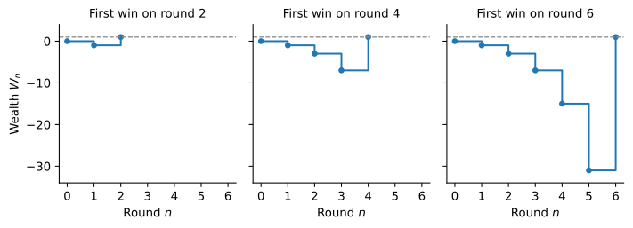
The doubling strategy bets one dollar on a fair coin, doubles the stake after every loss, and stops at the first win. If the first win comes on round k, the gambler has lost 2^{k - 1} - 1 dollars and then wins 2^{k - 1}, a net gain of one dollar, as in Figure 1. A win comes with probability one, yet over any n rounds \operatorname{E}(W_{n}) = (1 - 2^{-n}) - 2^{-n}(2^{n} - 1) = 0. The sure profit is paid for by an unbounded line of credit.
Stopping Times and Stopped Martingales
A random time \tau with values in \{0, 1, 2, \ldots\} \cup \{\infty\} is a stopping time if \{\tau \leq n\} \in \mathcal{F}_{n} for every n: whether we have stopped by time n is known at time n. The truncated time n \land \tau = \min\{n, \tau\} is always finite, and the stopped process M_{n \land \tau} freezes M at time \tau. Stopping is itself a betting strategy, one dollar per round while the game runs and nothing afterwards: M_{n \land \tau} = M_{0} + \sum_{k = 1}^{n} \mathbf{1}_{\{\tau \geq k\}} (M_{k} - M_{k - 1}). \tag{3} The stake \mathbf{1}_{\{\tau \geq k\}} is predictable because \{\tau \geq k\} is the complement of \{\tau \leq k - 1\} \in \mathcal{F}_{k - 1}, so a stopped martingale is a martingale and \operatorname{E}(M_{n \land \tau}) = \operatorname{E}(M_{0}) for every n.
Optional Stopping
If \tau is finite, M_{n \land \tau} \to M_{\tau} as n \to \infty, but the expectations need not converge: the doubling strategy has W_{\tau} = 1 and W_{0} = 0.
The doubling strategy fails the condition: the wealth just before the win is -(2^{\tau - 1} - 1), and \operatorname{E}(2^{\tau - 1}) = \sum_{k} 2^{k - 1} 2^{-k} = \infty.
Ruin Probabilities Again
For the fair random walk with S_{0} = 0 and \tau = \min\{n > 0 : S_{n} = A \text{ or } S_{n} = -B\}, the stopped walk is bounded by \max(A, B), so optional stopping gives \operatorname{E}(S_{\tau}) = 0, that is, A \operatorname{P}(S_{\tau} = A) - B (1 - \operatorname{P}(S_{\tau} = A)) = 0 and \operatorname{P}(S_{\tau} = A) = B / (A + B). The martingale S_{n}^{2} - n is dominated by \max(A^{2}, B^{2}) + \tau, which is integrable because \operatorname{E}(\tau) < \infty, so \operatorname{E}(S_{\tau}^{2}) = \operatorname{E}(\tau), which gives \operatorname{E}(\tau) = AB.
With a biased coin, S_{n} is not a martingale, but each factor (q / p)^{X_{i}} is positive with mean p \frac{q}{p} + q \frac{p}{q} = 1, so the product (q / p)^{S_{n}} is a martingale, bounded between (q / p)^{-B} and (q / p)^{A} when stopped. Optional stopping, together with the martingale S_{n} - n (p - q), gives P_{A} = \operatorname{P}(S_{\tau} = A) = \frac{(q / p)^{B} - 1}{(q / p)^{A + B} - 1}, \qquad \operatorname{E}(\tau) = \frac{A P_{A} - B (1 - P_{A})}{p - q}. \tag{5} The same pattern returns with Poisson processes and Brownian motion: an exponential martingale delivers the ruin probability.
Practice Problems
Let X_{1}, X_{2}, \ldots be independent fair coin flips, equal to 1 or -1 with probability 1/2, let S_{0} = 0, S_{n} = X_{1} + \cdots + X_{n}, and let \mathcal{F}_{n} be generated by X_{1}, \ldots, X_{n}.
- Compute \operatorname{E}(S_{n + 1}^{2} \mid \mathcal{F}_{n}). Is \{S_{n}^{2}\} a martingale?
- Show that \{S_{n}^{3} - 3 n S_{n}\} is a martingale.
- Find the constant c such that \{c^{n} 2^{S_{n}}\} is a martingale.
NoteSolution- \operatorname{E}(S_{n + 1}^{2} \mid \mathcal{F}_{n}) = S_{n}^{2} + 2 S_{n} \operatorname{E}(X_{n + 1}) + \operatorname{E}(X_{n + 1}^{2}) = S_{n}^{2} + 1. It exceeds S_{n}^{2}, so \{S_{n}^{2}\} is not a martingale: it drifts up by one each period, which is why S_{n}^{2} - n is.
- Using \operatorname{E}(X) = \operatorname{E}(X^{3}) = 0 and \operatorname{E}(X^{2}) = 1, \operatorname{E}(S_{n + 1}^{3} \mid \mathcal{F}_{n}) = S_{n}^{3} + 3 S_{n}^{2} \operatorname{E}(X) + 3 S_{n} \operatorname{E}(X^{2}) + \operatorname{E}(X^{3}) = S_{n}^{3} + 3 S_{n}, so \operatorname{E}(S_{n + 1}^{3} - 3 (n + 1) S_{n + 1} \mid \mathcal{F}_{n}) = S_{n}^{3} + 3 S_{n} - 3 (n + 1) S_{n} = S_{n}^{3} - 3 n S_{n}.
- \operatorname{E}(c^{n + 1} 2^{S_{n + 1}} \mid \mathcal{F}_{n}) = c^{n} 2^{S_{n}} \, c \, \operatorname{E}(2^{X}) = c^{n} 2^{S_{n}} \, c \, \frac{1}{2} \left(2 + \frac{1}{2}\right), so we need c \cdot \frac{5}{4} = 1, that is, c = 4/5.
A stock trades at a price M_{0} = 100 that is a martingale. Each period the price rises or falls by $10 with probability 1/2, for two periods. A trader buys one share at time 0. If the price falls in the first period, the trader “buys the dip” and holds two shares over the second period; if it rises, the trader sells and holds nothing over the second period. The trader starts with W_{0} = 0 and borrows at zero interest to buy.
- Write down H_{1} and H_{2} and explain why the strategy is predictable.
- Compute W_{2} on each of the four price paths, the probability that the trader makes money, and \operatorname{E}(W_{2}).
- Compute \operatorname{E}(W_{2} \mid \mathcal{F}_{1}) after a fall in the first period, and compare it with W_{1}.
NoteSolution- H_{1} = 1, and H_{2} = 2 after a fall and H_{2} = 0 after a rise. The position for the second period depends only on the first price move, which is known when the position is chosen.
- W_{2} = H_{1} (M_{1} - M_{0}) + H_{2} (M_{2} - M_{1}). After up-up and up-down, W_{2} = 10. After down-up, W_{2} = -10 + 2 (10) = 10, and after down-down, W_{2} = -10 - 20 = -30. The trader makes money with probability 3/4, but \operatorname{E}(W_{2}) = \frac{3}{4} (10) + \frac{1}{4} (-30) = 0.
- After a fall, W_{1} = -10 and \operatorname{E}(W_{2} \mid \mathcal{F}_{1}) = -10 + 2 \operatorname{E}(M_{2} - M_{1} \mid \mathcal{F}_{1}) = -10 = W_{1}. Buying the dip changes the shape of the payoff, frequent small gains against a rare large loss, but not its expected value.
A market maker’s inventory changes each period by +1, 0 or -1 with probability 1/3 each, independently, starting from zero. The market maker hedges as soon as the inventory reaches +4 or -2. Assume \tau is finite with \operatorname{E}(\tau) < \infty.
- Show that the inventory S_{n} is a martingale and find \sigma^{2} such that S_{n}^{2} - n \sigma^{2} is a martingale.
- Use optional stopping to compute the probability that the inventory reaches +4 first.
- Use optional stopping to compute the expected number of periods until the market maker hedges. Explain why it differs from AB = 8.
NoteSolution- Each step has mean \frac{1}{3} (1 + 0 - 1) = 0 and is independent of the past, so S_{n} is a martingale. With \sigma^{2} = \operatorname{E}(X^{2}) = 2/3, \operatorname{E}(S_{n + 1}^{2} \mid \mathcal{F}_{n}) = S_{n}^{2} + 2/3, so S_{n}^{2} - \frac{2}{3} n is a martingale.
- With A = 4 and B = 2, \operatorname{E}(S_{\tau}) = 0 gives 4 P_{A} - 2 (1 - P_{A}) = 0, so P_{A} = 1/3.
- \operatorname{E}(S_{\tau}^{2}) = \frac{2}{3} \operatorname{E}(\tau), and \operatorname{E}(S_{\tau}^{2}) = \frac{1}{3} (16) + \frac{2}{3} (4) = 8, so \operatorname{E}(\tau) = 12. It is AB / \sigma^{2}: the inventory moves in only two thirds of the periods, so reaching a barrier takes 3/2 times as long as for a coin that always moves.
A trader’s strategy gains $1 with probability p = 0.6 and loses $1 with probability q = 0.4 on each trade, independently. The trader stops after making $3 or after losing $3.
- Between which two values does the stopped martingale (q / p)^{S_{n \land \tau}} lie? Why does this matter for optional stopping?
- Use optional stopping to compute the probability that the trader makes $3 first.
- Use the martingale S_{n} - n (p - q) to compute the expected number of trades.
NoteSolution- The stopped walk stays between -3 and 3, and q / p = 2/3 < 1, so the stopped martingale lies between (2/3)^{3} = 8/27 and (2/3)^{-3} = 27/8. A bounded martingale satisfies the conditions of the optional stopping theorem, so \operatorname{E}((q / p)^{S_{\tau}}) = 1.
- P_{A} (2/3)^{3} + (1 - P_{A}) (2/3)^{-3} = 1 gives P_{A} = \frac{(3/2)^{3} - 1}{(3/2)^{3} - (2/3)^{3}} = \frac{1}{1 + (2/3)^{3}} = \frac{27}{35} = 0.771.
- \operatorname{E}(S_{\tau}) = (p - q) \operatorname{E}(\tau), so \operatorname{E}(\tau) = \frac{3 (27/35) - 3 (8/35)}{0.2} = \frac{57/35}{0.2} = 8.14 trades.