Class 8

Trading Gains and the Itô Integral

Throughout, \{B_{t}\} is a Brownian motion and \mathcal{F}_{t} is the information generated by its path up to time t. A process \{b_{t}\} is adapted if b_{t} is known given \mathcal{F}_{t}.

An investor who holds b_{t_{j}} units of an asset whose price is a Brownian motion from t_{j} to t_{j + 1}, choosing each position before seeing the next price change, earns I_{t} = \sum_{j = 0}^{n - 1} b_{t_{j}} \left(B_{t_{j + 1}} - B_{t_{j}}\right). \tag{1} The holding is evaluated at the left endpoint of each period. For a general adapted integrand, the Itô integral is the mean-square limit of these sums as the partition gets finer, \int_{0}^{t} b_{s} \mathop{}\!\mathrm{d}B_{s} = \lim_{\lVert{\Pi}\rVert \to 0} \sum_{j = 0}^{n - 1} b_{t_{j}} \left(B_{t_{j + 1}} - B_{t_{j}}\right). \tag{2} Because Brownian paths have infinite total variation, the evaluation point matters. Summing B_{t_{j}} \Delta B_{j} = \frac{1}{2} (B_{t_{j + 1}}^{2} - B_{t_{j}}^{2}) - \frac{1}{2} (\Delta B_{j})^{2}, the first term telescopes and the second converges to half the quadratic variation, so \int_{0}^{T} B_{s} \mathop{}\!\mathrm{d}B_{s} = \frac{1}{2} \left(B_{T}^{2} - T\right). \tag{3} The right endpoint would give \frac{1}{2} (B_{T}^{2} + T), the gains of an investor who picks each position after seeing the price move.

Properties of the Itô Integral

Each increment \Delta B_{j} has mean zero and is independent of \mathcal{F}_{t_{j}}, while b_{t_{j}} is known at t_{j}. From this single fact, if \operatorname{E}\left(\int_{0}^{t} b_{s}^{2} \mathop{}\!\mathrm{d}s\right) < \infty, then I_{t} = \int_{0}^{t} b_{s} \mathop{}\!\mathrm{d}B_{s} satisfies:

1. Martingale. \{I_{t}\} is a martingale with continuous paths, so \operatorname{E}(I_{t}) = 0.
2. Itô isometry. \operatorname{E}\left(I_{t}^{2}\right) = \operatorname{E}\left(\int_{0}^{t} b_{s}^{2} \mathop{}\!\mathrm{d}s\right).
3. Quadratic variation. [I, I]_{t} = \int_{0}^{t} b_{s}^{2} \mathop{}\!\mathrm{d}s.

A position of b_{s} units adds b_{s}^{2} \mathop{}\!\mathrm{d}s to the variance of the gains, and no strategy based on past information turns a fair game into a favorable one. When the integrand is a deterministic function f(s), each approximating sum is a sum of independent normals, so \int_{0}^{t} f(s) \mathop{}\!\mathrm{d}B_{s} \sim \mathcal{N}\left(0, \int_{0}^{t} f(s)^{2} \mathop{}\!\mathrm{d}s\right). \tag{4} If we only require \int_{0}^{t} b_{s}^{2} \mathop{}\!\mathrm{d}s < \infty path by path, the integral still has zero drift but may fail to be a martingale: it is a local martingale.

Itô Processes

An Itô process combines a time integral and an Itô integral, X_{t} = X_{0} + \int_{0}^{t} a_{s} \mathop{}\!\mathrm{d}s + \int_{0}^{t} b_{s} \mathop{}\!\mathrm{d}B_{s}, \qquad \mathop{}\!\mathrm{d}X_{t} = a_{t} \mathop{}\!\mathrm{d}t+ b_{t} \mathop{}\!\mathrm{d}B_{t}, \tag{5} with adapted drift a_{t} and volatility b_{t}. Over a short interval, \operatorname{E}(\mathop{}\!\mathrm{d}X_{t} \mid \mathcal{F}_{t}) = a_{t} \mathop{}\!\mathrm{d}t and \operatorname{V}(\mathop{}\!\mathrm{d}X_{t} \mid \mathcal{F}_{t}) = b_{t}^{2} \mathop{}\!\mathrm{d}t. Drift and volatility are determined by the paths, so an Itô process is a martingale only if its drift is zero. With the multiplication table (\mathop{}\!\mathrm{d}t)^{2} = 0, (\mathop{}\!\mathrm{d}t)(\mathop{}\!\mathrm{d}B_{t}) = 0 and (\mathop{}\!\mathrm{d}B_{t})^{2} = \mathop{}\!\mathrm{d}t, (\mathop{}\!\mathrm{d}X_{t})^{2} = b_{t}^{2} \mathop{}\!\mathrm{d}t, \qquad [X, X]_{t} = \int_{0}^{t} b_{s}^{2} \mathop{}\!\mathrm{d}s. The drift moves X by amounts of order \mathop{}\!\mathrm{d}t and leaves no trace in the quadratic variation.

Itô’s Formula

If f(x, t) is twice continuously differentiable in x and once in t, then Y_{t} = f(X_{t}, t) is an Itô process with \mathop{}\!\mathrm{d}Y_{t} = \frac{\partial f}{\partial t} \mathop{}\!\mathrm{d}t+ \frac{\partial f}{\partial x} \mathop{}\!\mathrm{d}X_{t} + \frac{1}{2} \frac{\partial^{2} f}{\partial x^{2}} (\mathop{}\!\mathrm{d}X_{t})^{2}. \tag{6} Substituting \mathop{}\!\mathrm{d}X_{t} and (\mathop{}\!\mathrm{d}X_{t})^{2} = b_{t}^{2} \mathop{}\!\mathrm{d}t, \mathop{}\!\mathrm{d}Y_{t} = \left(\frac{\partial f}{\partial t} + a_{t} \frac{\partial f}{\partial x} + \frac{1}{2} b_{t}^{2} \frac{\partial^{2} f}{\partial x^{2}}\right) \mathop{}\!\mathrm{d}t+ b_{t} \frac{\partial f}{\partial x} \mathop{}\!\mathrm{d}B_{t}. \tag{7} The term \frac{1}{2} b_{t}^{2} \frac{\partial^{2} f}{\partial x^{2}} \mathop{}\!\mathrm{d}t is the Itô correction. In practice, expand f to second order in \mathop{}\!\mathrm{d}X and first order in \mathop{}\!\mathrm{d}t, then simplify with the multiplication table. Three cases with X_{t} = B_{t}:

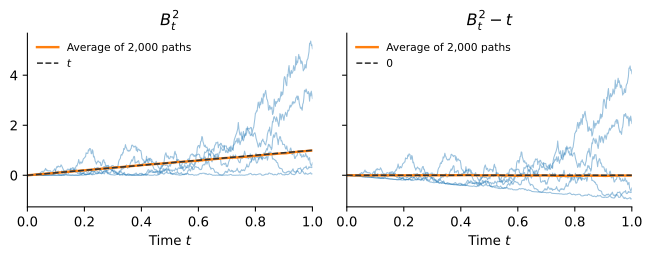
• \mathop{}\!\mathrm{d}(B_{t}^{2}) = 2 B_{t} \mathop{}\!\mathrm{d}B_{t} + \mathop{}\!\mathrm{d}t, which recovers (3) in one line. The drift of B_{t}^{2} is one, so B_{t}^{2} - t is a martingale, as Figure 1 shows.
• Z_{t} = \exp\left(\theta B_{t} - \frac{1}{2} \theta^{2} t\right) satisfies \mathop{}\!\mathrm{d}Z_{t} = \theta Z_{t} \mathop{}\!\mathrm{d}B_{t}: the Itô correction exactly offsets -\frac{1}{2} \theta^{2} t, so Z_{t} is a martingale.
• \mathop{}\!\mathrm{d}(t B_{t}) = B_{t} \mathop{}\!\mathrm{d}t+ t \mathop{}\!\mathrm{d}B_{t} has no correction, and gives \int_{0}^{T} B_{s} \mathop{}\!\mathrm{d}s = \int_{0}^{T} (T - s) \mathop{}\!\mathrm{d}B_{s} \sim \mathcal{N}(0, T^{3} / 3).

Since Itô integrals have mean zero, taking expectations of the integral form of Itô’s formula leaves only the drift: \operatorname{E}(Y_{t}) = Y_{0} + \operatorname{E}\left(\int_{0}^{t} \text{drift}_{s} \mathop{}\!\mathrm{d}s\right).

Figure 1: Five simulated paths of B_{t}^{2} and of B_{t}^{2} - t on [0, 1], with the average over 2,000 paths. Itô’s formula gives B_{t}^{2} a drift of one, so its average grows like t, while subtracting t removes the drift and leaves a martingale whose average stays at zero.

Practice Problems

1. The price of an asset follows a Brownian motion B_{t}, measured in dollars. A trader holds one unit from time 0 to time 1. At time 1 the trader looks at the price and, for the period from 1 to 2, holds two units if B_{1} > 0 and nothing otherwise. Let I_{2} be the trading gains at time 2.

   1. Write I_{2} as a sum of the form (1) and explain why the strategy is adapted.
   2. Compute \operatorname{E}(I_{2}) and \operatorname{E}(I_{2} \mid \mathcal{F}_{1}).
   3. Use the Itô isometry to compute \operatorname{V}(I_{2}).
   4. A second trader holds one unit from 0 to 1 and, for the period from 1 to 2, holds two units if B_{2} > B_{1} and nothing otherwise. Compute the expected gains of this trader and explain why this strategy is not allowed.
   NoteSolution

   1. I_{2} = 1 \cdot (B_{1} - B_{0}) + 2 \cdot \mathbf{1}_{\{B_{1} > 0\}} (B_{2} - B_{1}). Each position is chosen with the information available when it is taken: the second depends only on B_{1}, known at time 1.
   2. Each term has mean zero, because the position is known when the increment starts and the increment has mean zero, so \operatorname{E}(I_{2}) = 0. Given \mathcal{F}_{1}, the second term has mean zero, so \operatorname{E}(I_{2} \mid \mathcal{F}_{1}) = B_{1}.
   3. \operatorname{V}(I_{2}) = \operatorname{E}\left(\int_{0}^{2} b_{s}^{2} \mathop{}\!\mathrm{d}s\right) = 1 + 4 \operatorname{P}(B_{1} > 0) = 1 + 2 = 3.
   4. The gains are B_{1} + 2 \max(B_{2} - B_{1}, 0), and since B_{2} - B_{1} is standard normal, \operatorname{E}(\max(Z, 0)) = 1 / \sqrt{2 \pi} and the expected gain is 2 / \sqrt{2 \pi} = 0.80. The position over [1, 2] uses B_{2}, which is not known at time 1. The strategy is not adapted: it trades on the future.

2. A fund manager holds two units of an asset whose price follows a Brownian motion during the first half of the year and cuts the position to one unit for the second half. The gains over the year are I = \int_{0}^{1} f(s) \mathop{}\!\mathrm{d}B_{s}, with f(s) = 2 for s < \frac{1}{2} and f(s) = 1 for s \geq \frac{1}{2}.

   1. Find the distribution of I.
   2. Compute \operatorname{P}(I > 1).
   3. Compute \operatorname{Cov}(I, B_{1}) and the correlation between the gains and the price change over the year.
   NoteSolution

   1. The integrand is deterministic, so I is normal with mean zero and variance \int_{0}^{1} f(s)^{2} \mathop{}\!\mathrm{d}s = 4 \cdot \frac{1}{2} + 1 \cdot \frac{1}{2} = 2.5.
   2. \operatorname{P}(I > 1) = 1 - \mathop{\Phi}(1 / \sqrt{2.5}) = 1 - \mathop{\Phi}(0.63) = 0.264.
   3. B_{1} = \int_{0}^{1} 1 \mathop{}\!\mathrm{d}B_{s}, so by the Itô isometry \operatorname{Cov}(I, B_{1}) = \int_{0}^{1} f(s) \mathop{}\!\mathrm{d}s = 1 + \frac{1}{2} = 1.5, and the correlation is 1.5 / \sqrt{2.5} = 0.95.

3. Let X_{t} follow \mathop{}\!\mathrm{d}X_{t} = -\frac{1}{2} \kappa X_{t} \mathop{}\!\mathrm{d}t+ \frac{1}{2} \sigma \mathop{}\!\mathrm{d}B_{t}, with constants \kappa > 0 and \sigma > 0, and model the short-term interest rate as r_{t} = X_{t}^{2}.

   1. Use Itô’s formula to show that \mathop{}\!\mathrm{d}r_{t} = \kappa (\theta - r_{t}) \mathop{}\!\mathrm{d}t+ \sigma X_{t} \mathop{}\!\mathrm{d}B_{t}, and find \theta in terms of \kappa and \sigma.
   2. Show that (\mathop{}\!\mathrm{d}r_{t})^{2} = \sigma^{2} r_{t} \mathop{}\!\mathrm{d}t.
   3. With \kappa = 0.5 and \sigma = 0.2, compute \theta. When r_{t} = 4\%, compute the drift of the interest rate and the instantaneous standard deviation of \mathop{}\!\mathrm{d}r_{t} per unit of \sqrt{\mathop{}\!\mathrm{d}t}.
   NoteSolution

   1. With f(x) = x^{2}, \mathop{}\!\mathrm{d}r_{t} = 2 X_{t} \mathop{}\!\mathrm{d}X_{t} + (\mathop{}\!\mathrm{d}X_{t})^{2} and (\mathop{}\!\mathrm{d}X_{t})^{2} = \frac{1}{4} \sigma^{2} \mathop{}\!\mathrm{d}t, so \mathop{}\!\mathrm{d}r_{t} = \left(-\kappa X_{t}^{2} + \tfrac{1}{4} \sigma^{2}\right) \mathop{}\!\mathrm{d}t+ \sigma X_{t} \mathop{}\!\mathrm{d}B_{t} = \kappa (\theta - r_{t}) \mathop{}\!\mathrm{d}t+ \sigma X_{t} \mathop{}\!\mathrm{d}B_{t}, \qquad \theta = \frac{\sigma^{2}}{4 \kappa}.
   2. (\mathop{}\!\mathrm{d}r_{t})^{2} = \sigma^{2} X_{t}^{2} (\mathop{}\!\mathrm{d}B_{t})^{2} = \sigma^{2} r_{t} \mathop{}\!\mathrm{d}t. The volatility of the rate is proportional to \sqrt{r_{t}}, as in the model of Cox, Ingersoll and Ross.
   3. \theta = 0.04 / 2 = 2\%. At r_{t} = 4\% the drift is 0.5 (0.02 - 0.04) = -1\% per year, and the standard deviation per \sqrt{\mathop{}\!\mathrm{d}t} is \sigma \sqrt{r_{t}} = 0.2 \times 0.2 = 0.04.

4. Itô’s formula is also a tool for computing moments and finding martingales.

   1. Apply Itô’s formula to B_{t}^{4}, take expectations, and show that \operatorname{E}(B_{t}^{4}) = 3 t^{2}. Repeat the argument with B_{t}^{6} to compute \operatorname{E}(B_{t}^{6}).
   2. Show that M_{t} = e^{t / 2} \cos(B_{t}) has zero drift, and use this to compute \operatorname{E}(\cos(B_{t})).
   NoteSolution

   1. \mathop{}\!\mathrm{d}(B_{t}^{4}) = 4 B_{t}^{3} \mathop{}\!\mathrm{d}B_{t} + 6 B_{t}^{2} \mathop{}\!\mathrm{d}t. The Itô integral has mean zero, so \operatorname{E}(B_{t}^{4}) = 6 \int_{0}^{t} \operatorname{E}(B_{s}^{2}) \mathop{}\!\mathrm{d}s = 6 \int_{0}^{t} s \mathop{}\!\mathrm{d}s = 3 t^{2}. Likewise \mathop{}\!\mathrm{d}(B_{t}^{6}) = 6 B_{t}^{5} \mathop{}\!\mathrm{d}B_{t} + 15 B_{t}^{4} \mathop{}\!\mathrm{d}t, so \operatorname{E}(B_{t}^{6}) = 15 \int_{0}^{t} 3 s^{2} \mathop{}\!\mathrm{d}s = 15 t^{3}.
   2. By Itô’s formula, \mathop{}\!\mathrm{d}M_{t} = \tfrac{1}{2} e^{t / 2} \cos(B_{t}) \mathop{}\!\mathrm{d}t- e^{t / 2} \sin(B_{t}) \mathop{}\!\mathrm{d}B_{t} - \tfrac{1}{2} e^{t / 2} \cos(B_{t}) \mathop{}\!\mathrm{d}t= -e^{t / 2} \sin(B_{t}) \mathop{}\!\mathrm{d}B_{t}. The drift is zero and the integrand is bounded on [0, t], so M is a martingale and \operatorname{E}(M_{t}) = M_{0} = 1, that is, \operatorname{E}(\cos(B_{t})) = e^{-t / 2}.