Class 1

Payoff and Profit

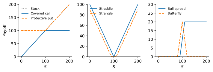
The options in this class are European and written on a stock that pays no dividends. Let S be the stock price at the maturity date T. A call with strike K pays \max(S - K, 0) and a put pays \max(K - S, 0), and a short position pays the negative of these amounts. An option strategy combines options with each other and with the stock, and its payoff is the sum of the payoffs of its legs. Ignoring interest on the premiums, \text{Profit} = \text{Payoff} - \text{Cost}, \qquad \text{Cost} = \text{premiums paid} - \text{premiums received}. \tag{1} A break-even price is a stock price at which the payoff equals the cost. The payoff of any strategy is piecewise linear in S, so the easiest way to find it is a table with one column for each interval between consecutive strikes. Reading the table from left to right, the slope of the payoff changes at each strike by the net number of options bought at that strike: a long call or a long put adds one, a short option subtracts one.

Strategy	Positions	Payoff at maturity
Covered call	Stock, short call K	\min(S, K)
Protective put	Stock, long put K	\max(S, K)
Collar	Stock, long put K_{1}, short call K_{2}	\min(\max(S, K_{1}), K_{2})
Straddle	Long call K, long put K	\lvert S - K \rvert
Strangle	Long put K_{1}, long call K_{2}	\max(K_{1} - S, 0) + \max(S - K_{2}, 0)
Bull spread	Long call K_{1}, short call K_{2}	\min(\max(S - K_{1}, 0), K_{2} - K_{1})
Bear spread	Long put K_{2}, short put K_{1}	\min(\max(K_{2} - S, 0), K_{2} - K_{1})
Butterfly	Long calls K_{1}, K_{3}; short 2 calls K_{2}	\max(K_{2} - K_{1} - \lvert S - K_{2} \rvert, 0)

The strikes satisfy K_{1} < K_{2} < K_{3}, and for the butterfly K_{2} = (K_{1} + K_{3}) / 2.

Stock and One Option

A covered call sells the upside above K in exchange for the call premium. It pays like the stock when S \leq K and is capped at K otherwise, so it beats holding the stock alone when the stock finishes near the strike, and it suits an investor who expects limited upside. A protective put buys insurance: the put floors the payoff at K, and the premium is the price of that floor. Since the two payoffs are \text{Covered call} = \min(S, K) \leq \max(S, K) = \text{Protective put}, \tag{2} no-arbitrage implies that a protective put never costs less than a covered call with the same strike and maturity. A collar adds both: the put floors the payoff at K_{1} and the short call caps it at K_{2}, so the investor keeps the stock with a bounded range of outcomes. When the strikes are chosen so that the two premiums are equal, the options cost nothing in total and the position is a zero-cost collar.

Betting on Volatility

A straddle buys a call and a put with the same strike. It pays \lvert S - K \rvert, so it profits from a large move in either direction and loses when the stock stays near the strike. With C and P the call and put premiums, the cost is C + P and the break-even prices are S = K - (C + P) \qquad \text{and} \qquad S = K + (C + P). \tag{3} A strangle buys a put with strike K_{1} and a call with strike K_{2} > K_{1}. Both options are further out of the money, so the strangle is cheaper than a straddle, but it pays nothing for any price between K_{1} and K_{2}. Its break-even prices are K_{1} minus the cost and K_{2} plus the cost. Both positions are bets on the size of the move, not its direction, and both lose value quickly if the move does not come.

Spreads and No-Arbitrage Bounds

A spread combines options of the same type on the same stock at different strikes, which caps both the gain and the loss. Write C_{i} and P_{i} for the prices of a call and a put with strike K_{i} and the same maturity. A bull spread buys the call with strike K_{1} and sells the call with strike K_{2}, so it pays between 0 and K_{2} - K_{1} and gains when the stock rises. A bear spread buys the put with strike K_{2} and sells the put with strike K_{1}, and gains when the stock falls. A butterfly pays only if the stock finishes near K_{2}, with a maximum payoff of K_{2} - K_{1} at S = K_{2}. It takes a view similar to a short straddle, but it costs money up front and the loss is limited to that cost. A condor buys calls at K_{1} and K_{4} and sells calls at K_{2} and K_{3}, with K_{2} - K_{1} = K_{4} - K_{3}, and pays K_{2} - K_{1} over the whole range [K_{2}, K_{3}].

None of these payoffs is ever negative, so none of the positions can have a negative cost: otherwise an investor would be paid today to take a position that never loses money at maturity. This gives three restrictions on option prices across strikes: C_{1} \geq C_{2}, \qquad P_{2} \geq P_{1}, \qquad C_{2} \leq \frac{C_{1} + C_{3}}{2} \quad \text{and} \quad P_{2} \leq \frac{P_{1} + P_{3}}{2}. \tag{4} Call prices fall with the strike, put prices rise with it, and both are convex functions of the strike. The butterfly can be built with puts as well as calls, with the same payoff, so P_{1} - 2 P_{2} + P_{3} = C_{1} - 2 C_{2} + C_{3} \geq 0. A quote that violates (4) is an arbitrage: buy the spread, collect the negative cost today, and keep a payoff that is never negative.

Figure 1: Payoffs at maturity against the stock price S. Left: stock, covered call and protective put with K = 100. Center: straddle with K = 100 and strangle with strikes 90 and 110. Right: bull spread with strikes 90 and 110 and butterfly with strikes 80, 100 and 120.

Why Stock Prices Are Lognormal

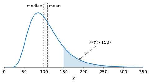
The continuously compounded return of a stock over [0, T] is R = \ln(S_{T} / S_{0}). Splitting the period into many short subperiods with returns R_{1}, \ldots, R_{n}, continuously compounded returns add up, R = \ln\left(\frac{S_{T}}{S_{0}}\right) = R_{1} + R_{2} + \cdots + R_{n}, \qquad S_{T} = S_{0} e^{R}. \tag{5} If the subperiod returns are independent and none dominates, the central limit theorem makes R approximately normal, and S_{T} is then the exponential of a normal random variable: a lognormal random variable. It is always positive, consistent with limited liability, and skewed to the right, since a stock can lose at most all of its value but can gain several times its value. The binomial tree has the same structure, since each period multiplies the price by u or d.

Normal and Lognormal Probabilities

If X \sim \mathcal{N}(\mu, \sigma^{2}), then X = \mu + \sigma Z with Z \sim \mathcal{N}(0, 1), and every probability about X is a value of the standard normal CDF \mathop{\Phi}. If Y = e^{X}, then Y is lognormal with parameters \mu and \sigma^{2}, which are the mean and variance of \ln(Y), not of Y. Since the logarithm is increasing, \begin{gathered} \operatorname{P}(X \leq x) = \mathop{\Phi}\left(\frac{x - \mu}{\sigma}\right), \qquad \mathop{\Phi}(-z) = 1 - \mathop{\Phi}(z), \\ \operatorname{P}(Y \leq y) = \operatorname{P}(X \leq \ln(y)) = \mathop{\Phi}\left(\frac{\ln(y) - \mu}{\sigma}\right). \end{gathered} \tag{6} The (1 - \alpha) probability interval for X is [\mu - z_{\alpha/2} \sigma, \mu + z_{\alpha/2} \sigma], where \operatorname{P}(Z > z_{\alpha/2}) = \alpha/2 (z_{0.05} = 1.645, z_{0.025} = 1.960, z_{0.005} = 2.576). Exponentiating the endpoints gives the interval for Y, which is not symmetric around e^{\mu}.

The moments follow from one formula, the expected exponential of a normal random variable. Since Y^{a} = e^{a X}, for any constant a, \operatorname{E}\left(e^{a X}\right) = \operatorname{E}(Y^{a}) = e^{a \mu + \frac{1}{2} a^{2} \sigma^{2}}, \qquad \operatorname{E}(Y) = e^{\mu + \frac{1}{2} \sigma^{2}}, \qquad \operatorname{SD}(Y) = \operatorname{E}(Y) \sqrt{e^{\sigma^{2}} - 1}. \tag{7} The term \frac{1}{2} \sigma^{2} comes from the convexity of e^{x}. Half of the distribution of \ln(Y) lies below \mu, so the median of Y is e^{\mu}, below the mean e^{\mu + \frac{1}{2} \sigma^{2}}: a few very large outcomes pull the mean above the typical value, and Y falls below its mean with probability \mathop{\Phi}(\frac{1}{2} \sigma) > \frac{1}{2}.

Figure 2: Lognormal density with \mu = \ln(100) and \sigma = 0.4. The dotted line marks the median e^{\mu} = 100 and the dashed line the mean e^{\mu + \frac{1}{2} \sigma^{2}} = 108.3. The shaded area is \operatorname{P}(Y > 150) = \mathop{\Phi}(d) = 0.155.

Partial Expectations

A call on Y with strike K pays \max(Y - K, 0) = Y \mathbf{1}_{\{Y > K\}} - K \mathbf{1}_{\{Y > K\}}, where the indicator \mathbf{1}_{\{Y > K\}} equals one if Y > K and zero otherwise. Its expected value needs two partial expectations, which average Y and K only over the outcomes where the option is exercised. With d = \frac{\mu - \ln(K)}{\sigma}, \qquad \operatorname{P}(Y > K) = \mathop{\Phi}(d), \qquad \operatorname{E}\left(Y \mathbf{1}_{\{Y > K\}}\right) = \operatorname{E}(Y) \mathop{\Phi}(d + \sigma), \tag{8} the expected payoff of the call is \operatorname{E}\left(\max(Y - K, 0)\right) = \operatorname{E}(Y) \mathop{\Phi}(d + \sigma) - K \mathop{\Phi}(d). \tag{9} The first term is the full mean of Y times a probability whose argument is shifted from d to d + \sigma: weighting each outcome by Y = e^{\mu + \sigma Z} gives more weight to high values of Z, as if Z were shifted to the right by \sigma. The Black-Scholes formula has exactly this form: it is the expected payoff of the call under a particular lognormal distribution, discounted at the risk-free rate.

Practice Problems

1. A stock trades for $64. Three-month European options on the stock trade at the following prices: a call with strike $70 costs $2.40 and a put with strike $58 costs $2.10.

   1. Compute the profit per share of a covered call with strike $70 if the stock price at maturity is $50, $64, $70 and $80. Find its break-even price and its maximum profit.
   2. Compute the cost of a collar that buys the put with strike $58 and writes the call with strike $70, and its profit per share for the same four stock prices. Find its maximum loss and its maximum profit.
   3. Explain which of the two positions fits an investor who wants to hold the stock through a period of possible large losses.

2. A dealer quotes the following prices for three-month European options on the same stock.

   Strike	Call	Put
   $90	$14.00	$3.10
   $100	$8.50	$5.20
   $110	$2.60	$9.30

   1. Check the call prices against each of the restrictions in (4). Which one is violated?
   2. Describe a trade with calls that exploits the violation. Compute the cash received today and the payoff at maturity for S \leq 90, 90 < S \leq 100, 100 < S \leq 110 and S > 110.
   3. Check the put prices against the same restrictions. Are they consistent with no-arbitrage?

3. A stock trades for $45 the day before it reports earnings. One-week European options with strike $45 trade at $2.30 for the call and $2.05 for the put.

   1. Compute the cost and the two break-even prices of a long straddle with strike $45. By how many percent must the stock move for the straddle to make money?
   2. Suppose that the stock price in one week is lognormal with \ln(S_{T}) \sim \mathcal{N}(\ln(45), 0.08^{2}). Compute the probability that the straddle makes a profit.
   3. A trader thinks the market overstates the size of the earnings move. Which position in the options expresses that view, and what are its maximum profit and maximum loss?

4. A stock trades for $80 today, and its price in one year satisfies \ln(S_{1}) \sim \mathcal{N}(\ln(80) + 0.04, \, 0.35^{2}).

   1. Compute the probability that S_{1} > 100 and the probability that the stock loses money over the year.
   2. Compute the median, the mean and the standard deviation of S_{1}.
   3. Compute the 90% probability interval for S_{1}. How far is each endpoint from the median, in dollars? Explain the asymmetry.

5. Let Y = e^{X} with X \sim \mathcal{N}(4.65, 0.25^{2}).

   1. Compute \operatorname{E}(Y), \operatorname{P}(Y > 110) and \operatorname{E}(Y \mathbf{1}_{\{Y > 110\}}).
   2. Compute the expected payoff \operatorname{E}(\max(Y - 110, 0)) of a call on Y with strike 110.
   3. Show that \max(110 - Y, 0) = \max(Y - 110, 0) - Y + 110 for every value of Y, and use it to compute the expected payoff of a put on Y with strike 110.