Class 4

Assets Paying a Dividend Yield

Stock indices and currencies pay their holders a steady stream of income, which we model as a continuous dividend yield \delta: over a short interval \Delta t, one unit of the asset bought for S_{t} pays \delta S_{t} \Delta t dollars, a payment known at t. The total return is the capital gain plus the dividend, \Delta S_{t} / S_{t} + \delta \Delta t.

A desk that sold a European option V on S replicates it with N_{S} units of the asset and N_{Z} zero-coupon bonds, so V = N_{S} S + N_{Z} Z. The asset now also pays dividends, and with dZ = r Z dt and N_{Z} Z = V - N_{S} S, the self-financing portfolio changes by dV = N_{S} (dS + \delta S dt) + N_{Z} dZ = \left(r V - (r - \delta) N_{S} S\right) dt + N_{S} dS. \tag{1} Matching this with Itô’s lemma for V(S, t) requires N_{S} = \partial V / \partial S, as without dividends, and leaves the Black-Scholes PDE with a dividend yield, \frac{1}{2} \sigma^{2} S^{2} \frac{\partial^{2} V}{\partial S^{2}} + (r - \delta) S \frac{\partial V}{\partial S} + \frac{\partial V}{\partial t} - r V = 0, \qquad V(S, T) = \text{payoff}. \tag{2} The PDE holds for derivatives that pay no dividends themselves; the asset S does not satisfy it.

The expected return of S never enters, so we may price in a risk-neutral world where every asset earns r in total. The dividend pays \delta of that return, so the price itself grows at r - \delta: dS = (r - \delta) S dt + \sigma S dB^{*}, \qquad \operatorname{E}^{*}(S_{T}) = S e^{(r - \delta) T}. \tag{3} A forward contract with delivery price K is worth e^{-r T} \operatorname{E}^{*}(S_{T} - K) = S e^{-\delta T} - K e^{-r T}, and setting this to zero gives the forward price F = S e^{(r - \delta) T}.

The Black-Scholes Formula with a Dividend Yield

Discounting the expected payoffs under (3) gives C = S e^{-\delta T} \mathop{\Phi}(d_{1}) - K e^{-r T} \mathop{\Phi}(d_{2}), \qquad P = K e^{-r T} \mathop{\Phi}(-d_{2}) - S e^{-\delta T} \mathop{\Phi}(-d_{1}), \tag{4} with d_{1} = \frac{\ln(S / K) + \left(r - \delta + \frac{1}{2} \sigma^{2}\right) T}{\sigma \sqrt{T}}, \qquad d_{2} = d_{1} - \sigma \sqrt{T}. The formula is the no-dividend Black-Scholes formula with S replaced by S e^{-\delta T}, the price today of receiving one unit of the asset at T without its dividends. Put-call parity reads C - P = S e^{-\delta T} - K e^{-r T}. The replicating portfolio of the call is N_{S} = \frac{\partial C}{\partial S} = e^{-\delta T} \mathop{\Phi}(d_{1}), \qquad N_{Z} = -\mathop{\Phi}(d_{2}), \tag{5} with N_{Z} counting bonds of face value K, and the delta of the put is \partial P / \partial S = -e^{-\delta T} \mathop{\Phi}(-d_{1}). The desk needs fewer units than without dividends because the dividends, reinvested in the asset, make the position grow at the rate \delta.

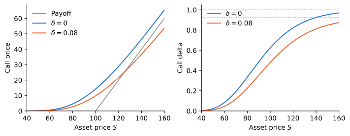
Dividends go to the holder of the asset, not to the holder of the call, so a positive yield lowers the call price and raises the put price. The lower bound of a European call is now S e^{-\delta T} - K e^{-r T}, whose slope e^{-\delta T} is less than one, so a deep in-the-money call falls below its exercise value S - K, as Figure 1 shows. The holder of an American call would rather exercise and collect the dividends.

Figure 1: Left: price of a one-year European call with strike K = 100, r = 0.05, and \sigma = 0.30, for an asset that pays no dividends and for one with \delta = 0.08, together with the payoff \max(S - K, 0). Right: the call delta e^{-\delta T} \mathop{\Phi}(d_{1}), with dotted lines at its limits 1 and e^{-0.08}.

Options on Stock Indices

An index such as the S&P 500 does not reinvest its dividends, so a portfolio that tracks it pays the index dividend yield \delta, and (4) prices options on the index with S the index level. SPX options, among the most liquid options in the world, are European, cash settled, and written on 100 times the index. Holding the stocks of the index involves no storage and no deterioration, and its only carry is the interest rate and the dividend yield, so carry arbitrage holds: index arbitrage keeps the futures price at the cash index plus carry, F = S e^{(r - \delta) T}.

Options on Currencies

Let S be the price of one unit of the base currency in the quote currency, such as dollars per euro for EUR/USD, with r the quote-currency rate and r_{f} the base-currency rate. A euro on deposit earns r_{f} exactly as an index earns its dividend yield, and holding it is riskless, so the desk replicates with N_{S} euros on deposit and N_{Z} dollar bonds, and everything above holds with \delta = r_{f}: dS = (r - r_{f}) S dt + \sigma S dB^{*}, \qquad F = S e^{(r - r_{f}) T}. \tag{6} The forward price is covered interest parity, and (4) with r_{f} in place of \delta is the model of Garman and Kohlhagen. A call on one currency is a put on the other: the right to buy €1 million for $1.25 million is the right to sell $1.25 million for €1 million, a put on USD/EUR with strike €0.80. Traders therefore name both currencies, as in EUR call / USD put. An option struck at the forward, K = F, is at-the-money-forward, and parity gives C = P.

Options on Futures

A call on a futures contract gives, on exercise, a long futures position plus the cash difference between the latest settlement price and the strike; a put gives a short position plus the difference between the strike and the settlement price. Let F be the futures price, with volatility \sigma. The desk replicates with N_{F} futures contracts and N_{Z} bonds, but entering a futures costs nothing: the contracts are marked to market and only pay N_{F} dF into the margin account. The portfolio value is all in the bond, V = N_{Z} Z, so dV = N_{F} dF + r V dt, \qquad N_{F} = \frac{\partial V}{\partial F}, \qquad \frac{1}{2} \sigma^{2} F^{2} \frac{\partial^{2} V}{\partial F^{2}} + \frac{\partial V}{\partial t} - r V = 0. \tag{7} This is (2) with \delta = r: a futures price behaves like an asset paying a dividend yield equal to the risk-free rate. Equivalently, a position that costs nothing and pays dF must have zero expected gain in a risk-neutral world, so F is a martingale, dF = \sigma F dB^{*}. Pricing the option as before gives Black’s model, C = e^{-r T} \left(F \mathop{\Phi}(d_{1}) - K \mathop{\Phi}(d_{2})\right), \qquad P = e^{-r T} \left(K \mathop{\Phi}(-d_{2}) - F \mathop{\Phi}(-d_{1})\right), \tag{8} with d_{1} = \frac{\ln(F / K) + \frac{1}{2} \sigma^{2} T}{\sigma \sqrt{T}}, \qquad d_{2} = d_{1} - \sigma \sqrt{T}. Put-call parity is C - P = e^{-r T} (F - K), and the call is hedged with N_{F} = e^{-r T} \mathop{\Phi}(d_{1}) futures contracts, the put with -e^{-r T} \mathop{\Phi}(-d_{1}). A deep in-the-money call approaches e^{-r T} (F - K), below its exercise value, so American futures options may be exercised early even though the futures pays no dividend.

Black’s Model in Practice

When the option expires with the futures, F_{T} = S_{T} and a futures option is an option on the underlying. For a financial underlying, substituting F = S e^{(r - \delta) T} into (8) gives back (4) exactly, since e^{-r T} F = S e^{-\delta T}, \qquad \ln(F / K) + \tfrac{1}{2} \sigma^{2} T = \ln(S / K) + \left(r - \delta + \tfrac{1}{2} \sigma^{2}\right) T. Currency traders often use the forward form anyway, because forward rates are quoted directly while the foreign rate behind them may not be observable on its own.

For a commodity no such substitution exists. The spot price of a commodity is the price of the nearby futures, the contract that trades and that dealers hedge with, and the cash price of the physical good is not tied to it by carry. The input to Black’s model is the futures price that matures with the option, read from the futures curve, and the desk hedges with that same contract.

Some exchanges list futures-style options: no premium changes hands, both sides post margin, and the option’s price is marked to market daily like a futures. Its futures price is the premium carried to maturity, \phi_{C} = C e^{r T} = F \mathop{\Phi}(d_{1}) - K \mathop{\Phi}(d_{2}), and similarly \phi_{P} = K \mathop{\Phi}(-d_{2}) - F \mathop{\Phi}(-d_{1}).

Practice Problems

1. An equity index stands at 5,000, has a dividend yield of 2% per year and a volatility of 20% per year, and the risk-free rate is 4% per year with continuous compounding. Consider six-month European options on the index with strike 5,000.

   1. Compute the six-month futures price of the index. Explain why carry arbitrage pins it down.
   2. Compute the prices of the call and the put, and check put-call parity.
   3. Find the units of the index and the bonds with face value 5,000 that replicate the call. How many units of the index would the desk hold if the index paid no dividends?
   4. A European call on the six-month index futures with strike 5,000 expires with the futures. Price it with Black’s model and compare it with the call in part (b). How many futures contracts replicate it per unit of the index, and why is this fewer than the units of the index in part (c)?

2. A US importer must pay £1,000,000 to a British supplier in three months. The GBP/USD spot rate is $1.30 per pound, its volatility is 10% per year, and the interest rates are 4% per year in dollars and 4.5% per year in pounds, both continuously compounded.

   1. Compute the three-month forward rate. Why is it below the spot rate?
   2. The importer buys a three-month GBP call / USD put with strike $1.32 per pound on £1,000,000. Compute the premium in dollars.
   3. A London bank sees the same contract as an option on USD/GBP, the price of one dollar in pounds. Is it a call or a put, and what are its strike and notional? Price it per dollar of notional, with pounds as the quote currency, and show that its d_{1} and d_{2} equal -d_{2} and -d_{1} from part (b). Check that its total value in pounds equals the dollar premium converted at the spot rate.
   4. At what strike would a three-month GBP call and GBP put have the same price?

3. A wire manufacturer will buy copper in three months and wants to cap its cost. The copper futures that expires in three months trades at $4.50 per pound with a volatility of 25% per year, each contract is written on 25,000 pounds, and the risk-free rate is 4% per year. The manufacturer buys 20 European calls on that futures with strike $4.75, expiring with the futures.

   1. Compute the price of the call per pound and the total premium.
   2. The dealer who sold the calls hedges with copper futures. How many contracts does it buy or sell?
   3. If the calls were futures-style options, what would be the futures price of a call per pound, and how much would the manufacturer pay for them today?
   4. The cash price of copper in a warehouse is $4.40 per pound. A colleague proposes to price the option from the cash price carried forward at the risk-free rate plus storage costs. Explain why the dealer uses the futures price instead.

4. An asset trades at $150, pays a dividend yield of 8% per year, and has a volatility of 20% per year. The risk-free rate is 3% per year.

   1. Compute the price of a one-year European call with strike $100 and compare it with the exercise value S - K.
   2. Compute the lower bound S e^{-\delta T} - K e^{-r T} and explain why the call can be worth less than its exercise value. What does this imply for an American call on the same asset?
   3. A one-year European call on a futures contract has strike $100, the futures trades at $150 with a volatility of 20% per year, and r = 3\%. Price it and compare it with F - K. Why can an American call on a futures be exercised early, even though the futures pays no dividends?

5. This problem uses the Black PDE in (7).

   1. Show that V(F, t) = e^{-r (T - t)} (F - K) satisfies the PDE. What payoff at T does it price?
   2. Show that V(F, t) = F does not satisfy the PDE, but V(F, t) = e^{-r (T - t)} F does. Explain the difference in terms of what a futures position costs.
   3. Show that V(S, t) = S e^{-\delta (T - t)} satisfies (2) and explain what it is the price of.