Class 3
The Replicating Portfolio
A trading desk has just sold a European option on a non-dividend-paying stock S, with maturity T and payoff F(S_{T}): \max(S_{T} - K, 0) for a call and \max(K - S_{T}, 0) for a put. The stock follows the geometric Brownian motion of the previous class, dS = \mu S dt + \sigma S dB. To hedge the short position, the traders hold N_{S} shares of the stock and N_{Z} zero-coupon bonds with face value K and maturity T, whose price Z = K e^{-r (T - t)} grows at the risk-free rate, dZ = r Z dt. The portfolio is worth V = N_{S} S + N_{Z} Z, and the goal is V_{T} = F(S_{T}).
The positions are rebalanced continuously, and each rebalancing is paid for with the value of the portfolio itself, so no money is added or withdrawn: the strategy is self-financing, as in the multi-period binomial tree. Its value then changes only because prices change. The bond position absorbs whatever is left after buying the shares, N_{Z} Z = V - N_{S} S, so dV = N_{S} dS + N_{Z} dZ = N_{S} dS + r (V - N_{S} S) dt. \tag{1}
Matching the Option
Let V(S, t) also denote the value of the option. By Itô’s lemma, with (dS)^{2} = \sigma^{2} S^{2} dt, dV = \frac{\partial V}{\partial S} dS + \left(\frac{1}{2} \sigma^{2} S^{2} \frac{\partial^{2} V}{\partial S^{2}} + \frac{\partial V}{\partial t}\right) dt. \tag{2} The hedge works when (1) and (2) agree. Matching the dS terms gives the number of shares, and matching the dt terms gives an equation for the option price: N_{S} = \frac{\partial V}{\partial S} = \Delta, \qquad \frac{1}{2} \sigma^{2} S^{2} \frac{\partial^{2} V}{\partial S^{2}} + r S \frac{\partial V}{\partial S} + \frac{\partial V}{\partial t} - r V = 0, \qquad V(S, T) = F(S). \tag{3} The number of shares in the hedge is the sensitivity of the option to the stock, its delta \Delta. The second equation is the Black-Scholes partial differential equation (PDE). Every derivative on S solves the same PDE and differs only in its payoff at T.
Risk-Neutral Pricing
The expected return \mu does not appear in (3). Holding \Delta shares cancels the dS terms, and with them any bet on the direction of the stock, just as the real probability of an up move never entered a binomial price. The option price is therefore the same in every economy with the same \sigma and r, whatever risk premium investors demand. In particular, it is the price in an economy of risk-neutral investors, where every asset earns the risk-free rate and the stock follows dS = r S dt + \sigma S dB^{*}. \tag{4} The asterisk marks a Brownian motion under the risk-neutral probabilities. The volatility is the same as under the real probabilities, since replication depends on it; only the drift changes. Itô’s lemma and (3) then give dV = r V dt + \sigma S \Delta dB^{*}, so the option also earns r on average, and its price is the expected payoff discounted at the risk-free rate: V = e^{-r T} \operatorname{E}^{*}\left(F(S_{T})\right). \tag{5} This shortcut is valid because the option can be replicated in the first place. It does not say that investors are risk neutral.
The Black-Scholes Formula
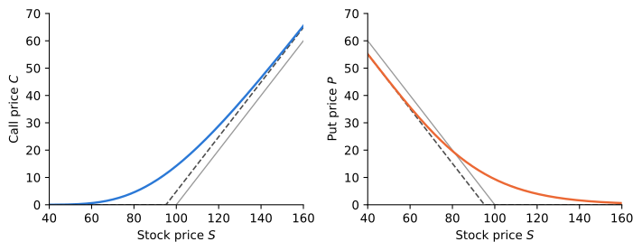
Under (4), \ln(S_{T}) is normal with mean \ln(S) + (r - \frac{1}{2} \sigma^{2}) T and variance \sigma^{2} T, where T now denotes the time to maturity. Splitting the call payoff as S_{T} \mathbf{1}_{\{S_{T} > K\}} - K \mathbf{1}_{\{S_{T} > K\}} and computing both partial expectations of the lognormal in (5) gives the Black-Scholes prices, with the put following from put-call parity C - P = S - K e^{-r T}: C = S \mathop{\Phi}(d_{1}) - K e^{-r T} \mathop{\Phi}(d_{2}), \qquad P = K e^{-r T} \mathop{\Phi}(-d_{2}) - S \mathop{\Phi}(-d_{1}), \tag{6} where d_{1} = \frac{\ln(S / K) + \left(r + \frac{1}{2} \sigma^{2}\right) T}{\sigma \sqrt{T}}, \qquad d_{2} = d_{1} - \sigma \sqrt{T}. \tag{7} Figure 1 plots both prices against the stock price. Each lies above its lower bound, \max(S - K e^{-r T}, 0) for the call and \max(K e^{-r T} - S, 0) for the put, and is convex in S.
Delta and the Replicating Portfolio
Differentiating (6) with respect to S gives the deltas, and writing each price as N_{S} S + N_{Z} Z with Z = K e^{-r T} reads off the bond positions: \text{Call: } \; N_{S} = \mathop{\Phi}(d_{1}), \quad N_{Z} = -\mathop{\Phi}(d_{2}), \qquad\qquad \text{Put: } \; N_{S} = -\mathop{\Phi}(-d_{1}), \quad N_{Z} = \mathop{\Phi}(-d_{2}). \tag{8} A call is a levered long position in the stock: buy \mathop{\Phi}(d_{1}) shares, financed partly by selling \mathop{\Phi}(d_{2}) bonds. A put is a short position in the stock with the proceeds invested in bonds. The call delta lies between 0 and 1 and the put delta between -1 and 0, and both deltas differ by exactly one, as put-call parity requires. As the stock moves, d_{1} changes and the desk must trade to keep N_{S} equal to the new delta: buying shares after the stock rises and selling after it falls.
The second partial expectation also gives the probability of exercise. Under the risk-neutral probabilities, \operatorname{P}^{*}(S_{T} > K) = \mathop{\Phi}(d_{2}), \qquad \operatorname{P}^{*}(S_{T} < K) = \mathop{\Phi}(-d_{2}). \tag{9} These are not forecasts. Under the real probabilities the stock grows at \mu, and the same calculation gives \operatorname{P}(S_{T} > K) = \mathop{\Phi}\big((\ln(S / K) + (\mu - \frac{1}{2} \sigma^{2}) T) / (\sigma \sqrt{T})\big), which exceeds \mathop{\Phi}(d_{2}) when \mu > r. Risk-neutral probabilities are implied by prices, like a bookmaker’s odds, not by a view on where the stock is going.
Example 1 A non-dividend-paying stock trades for $100, its volatility is 25% per year, and the risk-free rate is 4% per year with continuous compounding. For at-the-money options expiring in nine months, \begin{aligned} d_{1} &= \frac{\ln(100 / 100) + (0.04 + 0.5 \times 0.25^{2}) \times 0.75}{0.25 \sqrt{0.75}} = 0.2468, \\ d_{2} &= 0.2468 - 0.25 \sqrt{0.75} = 0.0303, \end{aligned} so \mathop{\Phi}(d_{1}) = 0.5975 and \mathop{\Phi}(d_{2}) = 0.5121, and \begin{aligned} C &= 100 \times 0.5975 - 100 e^{-0.04 \times 0.75} \times 0.5121 = \$10.05, \\ P &= 100 e^{-0.04 \times 0.75} \times 0.4879 - 100 \times 0.4025 = \$7.10. \end{aligned} To replicate the call, the desk buys 0.5975 shares and borrows 100 e^{-0.03} \times 0.5121 = \$49.70.
Volatility and Implied Volatility
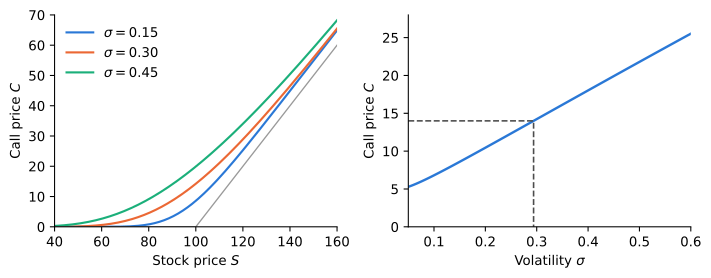
Both options gain value when volatility rises, by the same amount since C - P does not depend on \sigma: \frac{\partial C}{\partial \sigma} = \frac{\partial P}{\partial \sigma} = S \mathop{\Phi^{'}}(d_{1}) \sqrt{T} > 0, \qquad \mathop{\Phi^{'}}(d) = \frac{1}{\sqrt{2 \pi}} e^{-\frac{1}{2} d^{2}}. \tag{10} This sensitivity is the option’s vega. Because the price rises with \sigma one for one, a price can be quoted as a volatility. The implied volatility is the \sigma that makes (6) match the market price, C^{\text{mkt}} = C(\sigma_{\text{imp}}). It has no closed form and is found numerically, or by trial and error as in the right panel of Figure 2.
The model has a single volatility, so every option on the same stock should have the same implied volatility, whatever its strike and maturity. In practice it does not. For stock index options, implied volatility falls steeply with the strike (the volatility skew): deep out-of-the-money puts trade at much higher implied volatilities than at-the-money options. Index returns have a fatter left tail than the lognormal, volatility rises when prices fall, and replication is imperfect, so market makers who sell crash protection charge for the risk they cannot hedge. Traders still use the formula every day, as a translation device: they quote prices as implied volatilities, which can be compared across strikes, maturities, and underlying assets.
Practice Problems
A non-dividend-paying stock trades for $50 and has a volatility of 30% per year. The risk-free rate is 5% per year with continuous compounding. Consider European options on the stock with strike $48 that expire in six months.
- Compute d_{1} and d_{2}.
- Compute the price of the call and the price of the put.
- Verify that put-call parity holds.
- Compute the risk-neutral probability that each option is exercised.
The sales team of a desk sells 10 European call contracts, each on 100 shares, to a client. The stock pays no dividends and trades for $80, the strike is $85, the options expire in one year, the volatility is 35% per year, and the risk-free rate is 4% per year with continuous compounding.
- How many shares must the desk buy to hedge the sale?
- How many zero-coupon bonds with face value $85 and maturity one year must the desk hold, and how much money does it borrow?
- Check that the value of the replicating portfolio equals the premium the client pays.
- Suppose instead that the client bought 10 put contracts with the same terms. Find the positions N_{S} and N_{Z} of the hedge.
Two analysts follow a non-dividend-paying stock that trades for $100 and has a volatility of 20% per year. The first expects a return of 8% per year and the second 15% per year. The risk-free rate is 4% per year with continuous compounding. Consider a one-year European call with strike $110.
- Compute the price of the call. Does it depend on which analyst is right?
- Compute the risk-neutral probability that the call is exercised.
- Compute the probability of exercise according to each analyst, and explain the differences among the three probabilities.
A three-month at-the-money European call on a non-dividend-paying stock that trades for $100 sells for $5.00. The risk-free rate is 3% per year with continuous compounding.
- Compute the Black-Scholes price of the call for \sigma = 20\% and for \sigma = 25\%.
- Interpolate linearly between the two prices to estimate the implied volatility of the call.
- A three-month put on the same stock with strike $85 trades at an implied volatility of 32%. Is this consistent with the Black-Scholes model? Give an economic reason why the market might price the put this way.
Consider the options of Problem 1.
- Compute the vega of the call, S \mathop{\Phi^{'}}(d_{1}) \sqrt{T}.
- Volatility rises from 30% to 32%. Use the vega to estimate the new call and put prices.
- Explain, without differentiating the put formula, why the call and the put have the same vega.