Class 5

Delta and Hedging

The Black-Scholes model prices an option by replication: holding N_{S} = \partial V / \partial S shares and financing the rest with bonds reproduces the option when the position is rebalanced continuously. A desk that sells an option can hold the same portfolio as a hedge. In practice it rebalances at discrete times, once a day or once a week, and the Greeks measure what the position is exposed to between trades. For a portfolio of value V (stock, bonds, and options on the same underlying), the delta is \Delta = \frac{\partial V}{\partial S}, \qquad \Delta_{C} = e^{-\delta T} \mathop{\Phi}(d_{1}), \qquad \Delta_{P} = -e^{-\delta T} \mathop{\Phi}(-d_{1}), \tag{1} where, as in the Black-Scholes formula, d_{1} = \frac{\ln(S / K) + (r - \delta + \frac{1}{2} \sigma^{2}) T}{\sigma \sqrt{T}}, \qquad d_{2} = d_{1} - \sigma \sqrt{T}. The delta of a portfolio is the sum of the deltas of its positions. A share has a delta of one and a bond a delta of zero, so the desk sets the delta of its book by trading the stock. A book with \Delta = 0 is delta neutral. A desk short 5,000 calls with \Delta_{C} = 0.6 has a delta of -3{,}000 and buys 3,000 shares to neutralize it.

Gamma

Gamma is the rate at which delta changes with the stock price, and it is the reason a delta hedge must be rebalanced: \Gamma = \frac{\partial \Delta}{\partial S} = \frac{\partial^{2} V}{\partial S^{2}}, \qquad \Gamma_{C} = \Gamma_{P} = \frac{e^{-\delta T} \mathop{\Phi^{'}}(d_{1})}{S \sigma \sqrt{T}}, \qquad \mathop{\Phi^{'}}(x) = \frac{1}{\sqrt{2 \pi}} e^{-\frac{1}{2} x^{2}}. \tag{2} By Itô’s lemma, over a short interval \Delta t a portfolio changes by \Delta V \approx \Delta \cdot \Delta S + \frac{1}{2} \Gamma (\Delta S)^{2} + \Theta \Delta t, where \Theta = \partial V / \partial t is its theta. In a delta-neutral book the first term vanishes, \Delta V \approx \frac{1}{2} \Gamma (\Delta S)^{2} + \Theta \Delta t, \tag{3} so the book is not riskless: it moves with the square of the stock price change, and the sign of gamma decides whether large moves help or hurt. The stock and the bond have zero gamma, so gamma can only be changed by trading options. A delta-neutral book with \Gamma = 5{,}000 becomes gamma neutral by selling 5{,}000 / \Gamma_{C} calls, and then delta neutral again by buying \Delta_{C} shares per call sold.

Theta and the Profit of a Delta Hedge

The Black-Scholes equation ties the Greeks together. Written with them, it reads (r - \delta) S \Delta + \frac{1}{2} \sigma^{2} S^{2} \Gamma + \Theta = r V, \qquad \text{so} \qquad \frac{1}{2} \sigma^{2} S^{2} \Gamma + \Theta = r V \quad \text{when } \Delta = 0. \tag{4} In a delta-neutral book, a large positive theta comes with a large negative gamma and vice versa: theta is the price paid, or earned, for gamma. Substituting (4) into (3) and charging interest on the financed position, the profit over \Delta t of a long option hedged with \Delta shares is \frac{1}{2} \Gamma S^{2} \left[ \left(\frac{\Delta S}{S}\right)^{2} - \sigma^{2} \Delta t \right]. \tag{5} The bracket compares the squared return the stock delivered with the variance \sigma^{2} \Delta t used to price the option. A long-gamma position gains when the stock moves more than its volatility implies and loses its theta when it moves less. A desk that sold options earns theta in quiet markets and loses when the stock moves a lot. Over the life of the option, the hedged profit depends mainly on the volatility the stock actually realized relative to the \sigma in the price. Implied volatility on index options has historically exceeded the volatility realized afterwards, so desks that sell options and delta hedge collect a premium on average, as compensation for the large losses they take in crashes. Desks track this every day in a P&L attribution report that splits the profit into delta, gamma, theta, and vega parts.

Vega and Rho

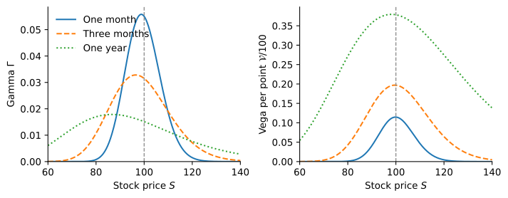
Vega is the sensitivity to volatility, computed in practice with respect to implied volatility, and rho is the sensitivity to the interest rate: \mathcal{V}_{C} = \mathcal{V}_{P} = S e^{-\delta T} \mathop{\Phi^{'}}(d_{1}) \sqrt{T}, \qquad \rho_{C} = K T e^{-r T} \mathop{\Phi}(d_{2}), \qquad \rho_{P} = -K T e^{-r T} \mathop{\Phi}(-d_{2}). \tag{6} The call has positive rho because it is a levered position in the stock financed by borrowing, and a higher rate lowers the value of the debt; the put combines a short stock position with lending. Like gamma, vega can only be hedged with options. Neutralizing gamma and vega at once takes two different options, with quantities N_{1} and N_{2} that solve \Gamma + N_{1} \Gamma_{1} + N_{2} \Gamma_{2} = 0, \qquad \mathcal{V} + N_{1} \mathcal{V}_{1} + N_{2} \mathcal{V}_{2} = 0, \tag{7} after which the stock restores delta neutrality. Theta follows from (4) as \Theta = r V - (r - \delta) S \Delta - \frac{1}{2} \sigma^{2} S^{2} \Gamma. Desks quote theta per day (\Theta / 365) and vega per volatility point (\mathcal{V} / 100). Figure 1 shows that gamma concentrates at the strike as expiration approaches, while vega grows with maturity: gamma risk dominates for short-dated options and vega risk for long-dated ones.

Figure 1: Gamma (left) and vega per volatility point (right) of a European call with K = 100, r = 5\%, \delta = 0, and \sigma = 25\%, against the stock price, for maturities of one month, three months, and one year. The dashed lines mark the strike.

Packages

A package is a portfolio of standard options sold as a single product. A long range forward sells a put with strike K_{1} and buys a call with strike K_{2} > K_{1}; a short range forward reverses both positions. The strikes are usually chosen so that the two premiums offset and the contract costs nothing. For an importer who must buy foreign currency at T, the long range forward caps the exchange rate paid at K_{2} and gives up any rate below K_{1}: \text{Price paid per unit} = S_{T} - \max(S_{T} - K_{2}, 0) + \max(K_{1} - S_{T}, 0) = \min\left(\max(S_{T}, K_{1}), K_{2}\right). \tag{8} It behaves like a long forward position that only locks the price within the range [K_{1}, K_{2}]. Its value is C(K_{2}) - P(K_{1}), both priced with Black-Scholes, and since C(F) = P(F) at the forward price, a zero-cost band always contains F: K_{1} < F < K_{2}.

Binary and Gap Options

A cash-or-nothing call pays Q if S_{T} > K, and an asset-or-nothing call pays one share if S_{T} > K. Their puts pay when S_{T} < K. A European call pays S_{T} - K when S_{T} > K, so it is long an asset-or-nothing call and short a cash-or-nothing call paying K, which is how the two terms of the Black-Scholes formula should be read: C = \underbrace{S e^{-\delta T} \mathop{\Phi}(d_{1})}_{\text{asset-or-nothing call}} - \underbrace{K e^{-r T} \mathop{\Phi}(d_{2})}_{\text{cash-or-nothing call}}. \tag{9} Likewise, a European put is long a cash-or-nothing put paying K and short an asset-or-nothing put. In general,

Type	Call	Put
Asset-or-nothing	S e^{-\delta T} \mathop{\Phi}(d_{1})	S e^{-\delta T} \mathop{\Phi}(-d_{1})
Cash-or-nothing	Q e^{-r T} \mathop{\Phi}(d_{2})	Q e^{-r T} \mathop{\Phi}(-d_{2})

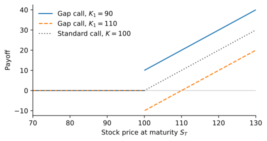
A gap call pays S_{T} - K_{1} when S_{T} > K_{2} and nothing otherwise: the trigger K_{2} decides whether the option pays and K_{1} decides how much. It is a long asset-or-nothing call and a short position in K_{1} cash-or-nothing calls paying $1, both triggered at K_{2}, and the gap put reverses the legs: \begin{aligned} \text{Gap Call} &= S e^{-\delta T} \mathop{\Phi}(d_{1}) - K_{1} e^{-r T} \mathop{\Phi}(d_{2}), \\ \text{Gap Put} &= K_{1} e^{-r T} \mathop{\Phi}(-d_{2}) - S e^{-\delta T} \mathop{\Phi}(-d_{1}), \end{aligned} \tag{10} with d_{1} and d_{2} computed at the trigger K_{2}. When K_{1} > K_{2} the payoff is negative for K_{2} < S_{T} < K_{1} (Figure 2), and the gap call can have a negative price.

Figure 2: Payoff at maturity of a gap call with trigger K_{2} = 100, for payment strikes K_{1} = 90 and K_{1} = 110. The dotted line is a standard call with strike 100.

Forward Start and Chooser Options

A forward start option is an at-the-money call or put that starts at \tau and expires at T > \tau, so its strike is K = S_{\tau}, as in many employee stock option plans. Since \ln(S_{\tau} / K) = 0 at the start date, d_{1} and d_{2} depend only on T - \tau, the option is worth a fixed number of shares at \tau, and \operatorname{E}^{*}(S_{\tau}) e^{-r \tau} = S e^{-\delta \tau} gives C = e^{-\delta \tau} \left( S e^{-\delta (T - \tau)} \mathop{\Phi}(d_{1}) - S e^{-r (T - \tau)} \mathop{\Phi}(d_{2}) \right), \qquad d_{1} = \frac{(r - \delta + \frac{1}{2} \sigma^{2}) (T - \tau)}{\sigma \sqrt{T - \tau}}. \tag{11} with d_{2} = d_{1} - \sigma \sqrt{T - \tau}. A forward start option is worth e^{-\delta \tau} times an at-the-money option with maturity T - \tau starting today; without dividends the two are equal. A cliquet is a series of forward start options, each starting when the previous one expires.

A chooser option lets the buyer decide at \tau whether it becomes a call or a put with strike K and maturity T. At \tau it is worth \max(C_{\tau}, P_{\tau}) = C_{\tau} + \max(P_{\tau} - C_{\tau}, 0), and put-call parity turns the second term into a put: \max(C_{\tau}, P_{\tau}) = C_{\tau} + e^{-\delta (T - \tau)} \max(\widetilde{K} - S_{\tau}, 0), \qquad \widetilde{K} = K e^{-(r - \delta) (T - \tau)}. \tag{12} The chooser is therefore a call with strike K and maturity T plus e^{-\delta (T - \tau)} puts with strike \widetilde{K} and maturity \tau, both priced with Black-Scholes. It costs less than a straddle, which pays both legs, and more than either a call or a put alone.

Practice Problems

1. A stock that pays no dividends trades at $80, its volatility is 30%, and the risk-free rate is 4% with continuous compounding. A desk has just sold 10,000 three-month at-the-money European calls.

   1. Compute d_{1}, the delta of one call, and the trade in the stock that makes the position delta neutral.
   2. Compute the gamma of one call.
   3. The next day the stock trades at $82. Use gamma to approximate the new delta of the position and the trade that restores delta neutrality.
   4. Compute the vega of the position per volatility point and its theta per calendar day at the original stock price. Explain their signs.

2. A dealer’s book is delta neutral, with a gamma of -1{,}000 and a vega of -6{,}000. Two traded options are available:

   	Delta	Gamma	Vega
   Option A	0.50	0.06	0.10
   Option B	0.40	0.02	0.25

   1. Make the book vega neutral using only Option B. What is the new gamma, and what trade in the stock restores delta neutrality?
   2. Make the book both gamma and vega neutral using Options A and B, and find the trade in the stock that restores delta neutrality.
   3. Explain why the dealer cannot use the stock to reduce gamma or vega.

3. A market maker’s options book is delta neutral and worth $10,000. The stock trades at $50, its volatility is 30%, the risk-free rate is 5%, and the gamma of the book is -400.

   1. Use (4) to compute the theta of the book per year and per calendar day.
   2. Use (5) to estimate the profit or loss of the book over one day in which the stock rises by $1.50.
   3. How large a daily move in the stock makes the book break even?
   4. Over the coming month, would the market maker rather see realized volatility above or below 30%? Explain.

4. A stock trades at $60, pays a dividend yield of 2%, and has a volatility of 25%. The risk-free rate is 5%. All options below mature in six months and are triggered at $65.

   1. Compute d_{1} and d_{2}, and price an asset-or-nothing call and a cash-or-nothing call that pays $10.
   2. Use (9) to price a standard European call with strike $65.
   3. Price a gap call that pays S_{T} - 60 if S_{T} > 65.
   4. Find the payment strike K_{1} that makes the gap call cost nothing today. Over which range of prices does its holder lose money at maturity?

5. A stock that pays no dividends trades at $40, its volatility is 35%, and the risk-free rate is 6%.

   1. Price an at-the-money forward start call that starts in three months and expires in one year.
   2. Explain why its price equals that of a nine-month at-the-money call bought today.
   3. Price a chooser option with strike $40 and maturity one year, where the holder chooses between the call and the put in three months.
   4. Price a one-year straddle with strike $40 and compare it with the chooser. Why is the chooser cheaper?

6. A U.S. importer must pay €1 million in six months. The six-month forward price is $1.10 per euro. A bank offers a zero-cost long range forward with strikes K_{1} = 1.05 and K_{2} = 1.154.

   1. Compute the dollar cost of the €1 million if the exchange rate in six months is 1.00, 1.10, or 1.20, and compare it with the cost under a forward contract.
   2. Use put-call parity to show that a zero-cost range forward must have the forward price between K_{1} and K_{2}.