Class 2

From Binomial Trees to Brownian Motion

A binomial tree with u = e^{\sigma \sqrt{\Delta t}} and d = 1 / u adds \sigma \sqrt{\Delta t} to the log price or subtracts it each period. After m periods, at time t = m \Delta t, with X_{i} = +1 for an up move and -1 for a down move, equally likely and independent, \ln(S_{t}) = \ln(S_{0}) + \sigma \sqrt{\Delta t} \, (X_{1} + X_{2} + \cdots + X_{m}), \qquad \operatorname{V}\left(\ln(S_{t})\right) = \sigma^{2} \Delta t \times m = \sigma^{2} t. \tag{1} The variance of the log price grows in proportion to time however short the periods are. This is why the steps scale with \sqrt{\Delta t}: steps proportional to \Delta t would freeze the price as \Delta t \to 0, and steps that do not shrink would make the variance explode.

Setting \sigma aside, the random part is the scaled random walk B_{t}^{(n)} = \sqrt{\Delta t} \, (X_{1} + \cdots + X_{m}), with n = 1 / \Delta t steps per unit of time, mean zero and variance t. As n \to \infty, the central limit theorem makes its value at t, and its change over any interval, normally distributed. The limit is a Brownian motion \{B_{t}\}, defined by four properties:

1. B_{0} = 0.
2. For s < t, the increment B_{t} - B_{s} is normal with mean zero and variance t - s.
3. Increments over non-overlapping intervals are independent.
4. The path t \mapsto B_{t} is continuous.

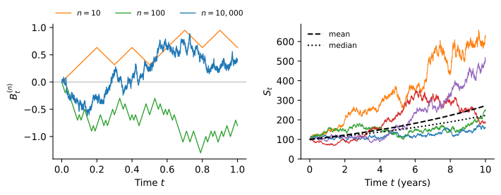
In particular B_{t} = \sqrt{t} \, Z for a standard normal Z. Over a short interval dt, the increment dB has standard deviation \sqrt{dt}, much larger than dt, so the path is continuous but nowhere smooth (Figure 1, left).

Geometric Brownian Motion

A Brownian motion can turn negative and its changes do not depend on its level, while a stock at $200 moves about twice as many dollars as the same stock at $100. What is roughly stable is the distribution of returns, so we let returns follow a Brownian motion with drift: \frac{dS}{S} = \mu \, dt + \sigma \, dB, \qquad \text{or} \qquad dS = \mu S \, dt + \sigma S \, dB. \tag{2} The process \{S_{t}\} is a geometric Brownian motion (GBM). The constant \mu is the expected return per unit of time and \sigma is the volatility of returns, the same \sigma used to build binomial trees, both quoted per year. The paths stay positive, their fluctuations grow with the price level, and they fan out unevenly (Figure 1, right).

Figure 1: Left: one path of the scaled random walk on [0, 1] with n = 10, 100 and 10{,}000 steps per unit of time. Right: five simulated GBM paths with S_{0} = 100, \mu = 0.10 and \sigma = 0.20; the dashed line is the expected price S_{0} e^{\mu t} and the dotted line the median price S_{0} e^{(\mu - \frac{1}{2} \sigma^{2}) t}.

Itô’s Lemma

In ordinary calculus, a smooth function changes by \Delta F \approx F'(x) \, \Delta x + \frac{1}{2} F''(x) (\Delta x)^{2}, and the second-order term is negligible. For a Brownian motion, (\Delta B)^{2} has mean \Delta t, the same order as the time step. Adding up the n squared increments of a path over [0, t] gives a sum with mean t and variance 2 t \, \Delta t \to 0, so the sum converges to t on every path. In differential notation, this is the multiplication table (dB)^{2} = dt, \qquad (dt)(dB) = 0, \qquad (dt)^{2} = 0, \qquad \text{so that} \qquad (dS)^{2} = \sigma^{2} S^{2} \, dt. \tag{3} Only the random term of the stock price contributes to (dS)^{2}. Expanding a function F(S, t) to second order in dS and first order in dt, and keeping (dS)^{2}, gives Itô’s lemma: dF = \frac{\partial F}{\partial S} \, dS + \frac{1}{2} \frac{\partial^{2} F}{\partial S^{2}} \, (dS)^{2} + \frac{\partial F}{\partial t} \, dt = \left(\mu S \frac{\partial F}{\partial S} + \frac{1}{2} \sigma^{2} S^{2} \frac{\partial^{2} F}{\partial S^{2}} + \frac{\partial F}{\partial t}\right) dt + \sigma S \frac{\partial F}{\partial S} \, dB. \tag{4} The term \frac{1}{2} \sigma^{2} S^{2} \frac{\partial^{2} F}{\partial S^{2}} is the Itô correction. It vanishes when \sigma = 0 or when F is linear in S. For example, the discounted price F = e^{-r t} S satisfies dF = (\mu - r) F \, dt + \sigma F \, dB, a GBM whose expected return is the risk premium \mu - r. More importantly, (4) shows that F is driven by the same dB as the stock, with a random term proportional to \partial F / \partial S. This common source of risk is what allows an option to be replicated with the stock in the Black-Scholes model.

Solving for the Stock Price

Applying (4) to F(S) = \ln(S), with \partial F / \partial S = 1 / S and \partial^{2} F / \partial S^{2} = -1 / S^{2}, d\ln(S) = \frac{dS}{S} - \frac{1}{2} \frac{(dS)^{2}}{S^{2}} = \left(\mu - \tfrac{1}{2} \sigma^{2}\right) dt + \sigma \, dB. The coefficients are constant, so the changes add up to \ln(S_{T}) - \ln(S_{0}) = \left(\mu - \frac{1}{2} \sigma^{2}\right) T + \sigma B_{T}, and S_{T} = S_{0} \exp\left(\left(\mu - \tfrac{1}{2} \sigma^{2}\right) T + \sigma B_{T}\right). \tag{5} The log price is a Brownian motion with drift \mu - \frac{1}{2} \sigma^{2}, the continuous-time version of the log price in a binomial tree. Ordinary calculus would have given it a drift of \mu.

The Distribution of the Stock Price

Since B_{T} \sim \mathcal{N}(0, T), (5) implies that S_{T} is lognormal, the distribution we studied in Class 1: \ln(S_{T}) \sim \mathcal{N}(m, s^{2}), \qquad m = \ln(S_{0}) + \left(\mu - \tfrac{1}{2} \sigma^{2}\right) T, \qquad s = \sigma \sqrt{T}. \tag{6} The continuously compounded return \ln(S_{T} / S_{0}) is normal with mean \left(\mu - \frac{1}{2} \sigma^{2}\right) T and standard deviation \sigma \sqrt{T}. To compute a probability about the price, translate it into a statement about the log price and standardize: \operatorname{P}(S_{T} \leq K) = \operatorname{P}\left(Z \leq \frac{\ln(K) - m}{s}\right) = \mathop{\Phi}\left(\frac{\ln(K / S_{0}) - \left(\mu - \frac{1}{2} \sigma^{2}\right) T}{\sigma \sqrt{T}}\right). \tag{7} A probability interval [m - z s, m + z s] for \ln(S_{T}) becomes the interval [e^{m - z s}, e^{m + z s}] for S_{T}, with z = 1.96 for 95%. It is not symmetric around the current price, because the lognormal distribution is skewed to the right. For instance, with S_{0} = 25, \mu = 12\%, \sigma = 25\% and T = 0.5, we get m = 3.2633 and s = 0.1768, and the 95% interval for the price in six months is [18.48, 36.96].

Moments, Median and Growth Rate

The lognormal moments \operatorname{E}(S_{T}) = e^{m + \frac{1}{2} s^{2}} and \operatorname{SD}(S_{T}) = \operatorname{E}(S_{T}) \sqrt{e^{s^{2}} - 1} give \operatorname{E}(S_{T}) = S_{0} e^{\mu T}, \qquad \operatorname{SD}(S_{T}) = \operatorname{E}(S_{T}) \sqrt{e^{\sigma^{2} T} - 1}. \tag{8} The expected price grows at the rate \mu, which is why \mu is called the expected return, and the uncertainty about the future price grows faster than its expected value. The median is the price at which the log price is at its mean, \text{Median}(S_{T}) = S_{0} e^{\left(\mu - \frac{1}{2} \sigma^{2}\right) T} < S_{0} e^{\mu T} = \operatorname{E}(S_{T}). \tag{9} Both growth rates are correct. A few paths that end very high pull the mean above what a typical path achieves, as the dashed and dotted lines in Figure 1 show. The rate \mu - \frac{1}{2} \sigma^{2} is what a long-term holder typically realizes, while \mu is the rate at which wealth grows on average across all paths. The price ends below its mean when \sigma B_{T} < \frac{1}{2} \sigma^{2} T, which has probability \mathop{\Phi}\left(\frac{1}{2} \sigma \sqrt{T}\right) > \frac{1}{2}.

The Black-Scholes model prices options with this lognormal distribution, with one change: the expected return \mu is replaced by the risk-free rate r. Next class explains why.

Practice Problems

1. A stock has a volatility of \sigma = 30\% per year, and up and down moves are equally likely in a binomial tree for its price.

   1. Compute u and d for a tree with monthly steps (\Delta t = 1/12) and for a tree with daily steps (\Delta t = 1/252).
   2. Use (1) to show that the variance of the one-year log return is the same in both trees, and compute it.
   3. Suppose instead that each step adds or subtracts \sigma \Delta t from the log price. Compute the standard deviation of the one-year log return with monthly and with daily steps, and explain what happens as \Delta t \to 0.

2. Let \{B_{t}\} be a Brownian motion, with time measured in years.

   1. Give the distribution of B_{4} - B_{1}, and compute \operatorname{P}(B_{4} - B_{1} > 2).
   2. Suppose you observe B_{1} = 0.5. Compute the probability that B_{4} > 0.
   3. You add up the 252 squared daily increments of a Brownian path over one year. Compute the mean and the standard deviation of the sum. Repeat with one-minute increments, assuming 390 minutes per trading day, and relate your answer to the rule (dB)^{2} = dt.

3. A stock pays no dividends and follows a GBM with \mu = 11\% and \sigma = 25\% per year. The risk-free rate is r = 4\% per year, continuously compounded. The forward price for delivery of the stock at time T is F(S, t) = S e^{r (T - t)}.

   1. Use Itô’s lemma to find dF, and give the expected return and the volatility of the forward price.
   2. Use Itô’s lemma to find d\ln(F).
   3. Since F_{T} = S_{T}, check that your answer to the previous part gives the same distribution for \ln(S_{T}) as (6).

4. A stock trades at $80 and follows a GBM with \mu = 14\% and \sigma = 40\% per year. Consider the price three months from now.

   1. Compute the expected value and the standard deviation of S_{T}.
   2. Compute the 90% probability interval for S_{T}, using z = 1.645. How far is each endpoint from the current price?
   3. Compute the probability that the stock trades below $70 in three months.

5. A stock follows a GBM with \mu = 8\% and \sigma = 40\% per year.

   1. Compute the growth rate of the log price. Compute the median and the expected value of S_{T} / S_{0} for T = 1, 10 and 30 years.
   2. Show that \operatorname{P}(S_{T} > S_{0}) does not depend on the horizon, and compute it.
   3. Compute \operatorname{P}\left(S_{T} > \operatorname{E}(S_{T})\right) for T = 1, 10 and 30 years. Explain how the expected price can grow elevenfold over 30 years while the typical investor ends where she started.