A First Neural Network

This notebook trains neural networks on two problems. In the first, a strong signal is hidden in noisy data, and the network finds it easily. In the second, we try to predict the stock market’s return from the variables Welch and Goyal (2008) study, and the network does badly on data it was not trained on. The second problem is the one finance actually poses, and seeing why the network fails is the point of the exercise.

Packages

PyTorch is the library we use to build and train networks. Fixing the random seed makes the results reproducible: training starts from random weights, and a different seed gives a somewhat different network.

from pathlib import Path

import matplotlib.pyplot as plt
import numpy as np
import pandas as pd
import torch
import torch.nn as nn

torch.manual_seed(0)
rng = np.random.default_rng(0)

An easy problem: learning a call payoff

We generate 1,000 stock prices and the payoff of a call option with strike 100 on each, plus noise. A linear regression cannot fit the kink at the strike; a network with a few hidden units can.

S = rng.uniform(60, 140, size=1000)
payoff = np.maximum(S - 100, 0) + rng.normal(scale=3, size=1000)

# Networks train best when inputs are of order one, so we rescale the price
X = torch.tensor((S[:, None] - 100) / 20, dtype=torch.float32)
Y = torch.tensor(payoff[:, None], dtype=torch.float32)

A network in PyTorch is a sequence of layers. This one takes one input, has a hidden layer of eight units with the ReLU activation, and produces one output.

net = nn.Sequential(
    nn.Linear(1, 8),
    nn.ReLU(),
    nn.Linear(8, 1),
)

Training is gradient descent on the mean squared error. Each pass computes the loss, computes its gradient with backward(), and lets the optimizer take a step.

opt = torch.optim.Adam(net.parameters(), lr=0.05)
for epoch in range(2000):
    opt.zero_grad()
    loss = ((net(X) - Y) ** 2).mean()
    loss.backward()
    opt.step()
print(f"Final training loss: {loss.item():.2f}")

Final training loss: 9.46

The noise we added has a variance of 3^2 = 9, so a loss close to 9 means the network has found the payoff and is left with the noise only.

grid = np.linspace(60, 140, 200)
with torch.no_grad():
    fit = net(torch.tensor((grid[:, None] - 100) / 20, dtype=torch.float32)).numpy().ravel()
b1, b0 = np.polyfit(S, payoff, 1)

fig, ax = plt.subplots(figsize=(7, 3.5))
ax.scatter(S, payoff, s=4, color="0.75", label="Data")
ax.plot(grid, b0 + b1 * grid, label="Linear regression")
ax.plot(grid, fit, label="Neural network")
ax.set_xlabel("Stock price")
ax.set_ylabel("Payoff")
ax.legend(frameon=False)
plt.show()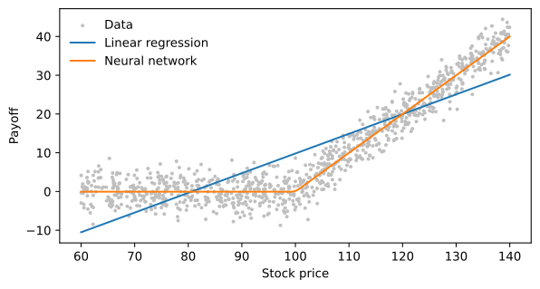

A hard problem: predicting the stock market

The data

Amit Goyal keeps the data of Welch and Goyal (2008) up to date on his website. The monthly file has the S&P 500, its dividends and earnings, interest rates, and other variables proposed as predictors of the market’s return. We download it once and save it.

DATA = Path("../_data") if Path("../_data").exists() else Path("data")
file = DATA / "goyal_welch_monthly_2025.parquet"
if not file.exists():
    url = ("https://docs.google.com/spreadsheets/d/"
           "1qwpl2R_DNujpU5YUkk8lacP1tTeMb9iJ/export?format=csv")
    DATA.mkdir(exist_ok=True)
    pd.read_csv(url, thousands=",").to_parquet(file)
raw = pd.read_parquet(file)
raw.index = pd.PeriodIndex(raw.pop("yyyymm").astype(str), freq="M")
raw.tail(3)

	Index	D12	E12	b/m	tbl	AAA	BAA	lty	ntis	Rfree	infl	ltr	corpr	svar	csp	CRSP_SPvw	CRSP_SPvwx
yyyymm
2025-10	6840.20	78.6242	238.1967	0.172936	0.0382	0.0513	0.0574	0.0406	-0.008996	0.0037	-0.001044	0.0062	0.0038	0.001646	NaN	0.023013	0.022302
2025-11	6849.09	78.7722	242.3333	0.172380	0.0378	0.0526	0.0586	0.0409	-0.008713	0.0030	-0.001045	0.0062	0.0065	0.001700	NaN	0.002286	0.001166
2025-12	6845.50	78.9202	246.4700	0.171136	0.0359	0.0531	0.0590	0.0414	-0.029750	0.0034	-0.000210	-0.0033	-0.0020	0.000649	NaN	0.000834	-0.000293

We build nine predictors as Welch and Goyal (2008) do: the dividend-price and earnings-price ratios of the S&P 500 (in logs), the book-to-market ratio of the Dow Jones, the Treasury bill rate, the term spread, the default spread, net equity issuance, stock variance, and inflation. Inflation is published with a delay, so we lag it one more month. The outcome is the next month’s equity premium: the return on the value-weighted CRSP index of S&P 500 stocks minus the Treasury bill rate.

X = pd.DataFrame({
    "dp": np.log(raw["D12"]) - np.log(raw["Index"]),
    "ep": np.log(raw["E12"]) - np.log(raw["Index"]),
    "bm": raw["b/m"],
    "tbl": raw["tbl"],
    "tms": raw["lty"] - raw["tbl"],
    "dfy": raw["BAA"] - raw["AAA"],
    "ntis": raw["ntis"],
    "svar": raw["svar"],
    "infl": raw["infl"].shift(1),
})
premium = (raw["CRSP_SPvw"] - raw["Rfree"]).shift(-1).rename("premium")
data = pd.concat([X, premium], axis=1).dropna()
predictors = list(X.columns)
print(data.index.min(), "to", data.index.max(), f"({len(data)} months)")

1926-12 to 2025-11 (1188 months)

Training, validation and test samples

We train on the months up to 1979, use 1980 to 1999 to decide when to stop training the network, and keep 2000 to 2025 for the final test. The test sample is never used to make any choice.

train = data.loc[:"1979-12"]
valid = data.loc["1980-01":"1999-12"]
test = data.loc["2000-01":]

# Standardize with the training sample's means and standard deviations only
mu, sd = train[predictors].mean(), train[predictors].std()
z = lambda df: ((df[predictors] - mu) / sd).to_numpy(dtype="float32")

The benchmark is the simplest forecast: the average premium in the training sample. A model is worth something only if it beats that. We measure this with the out-of-sample R^2, which compares a model’s squared forecast errors with the benchmark’s and is negative when the model does worse.

benchmark = train["premium"].mean()

def r2_oos(actual, forecast):
    return 1 - ((actual - forecast) ** 2).sum() / ((actual - benchmark) ** 2).sum()

Linear regressions

First, one predictor at a time, then all nine together, the “kitchen sink.”

def linear_forecasts(cols):
    A = np.c_[np.ones(len(train)), ((train[cols] - mu[cols]) / sd[cols])]
    beta = np.linalg.lstsq(A, train["premium"], rcond=None)[0]
    predict = lambda df: np.c_[np.ones(len(df)), ((df[cols] - mu[cols]) / sd[cols])] @ beta
    return predict

rows = []
for col in predictors + ["all nine"]:
    cols = predictors if col == "all nine" else [col]
    predict = linear_forecasts(cols)
    rows.append({"predictors": col,
                 "R2 train": 1 - ((train["premium"] - predict(train)) ** 2).sum()
                                 / ((train["premium"] - benchmark) ** 2).sum(),
                 "R2 test (2000-2025)": r2_oos(test["premium"], predict(test))})
pd.DataFrame(rows).set_index("predictors").round(3)

	R2 train	R2 test (2000-2025)
predictors
dp	0.010	-0.147
ep	0.009	-0.069
bm	0.021	-0.131
tbl	0.005	0.005
tms	0.002	-0.020
dfy	0.004	-0.004
ntis	0.011	-0.052
svar	0.002	-0.003
infl	0.003	-0.006
all nine	0.056	-0.490

A neural network

The network has one hidden layer of 16 units. We train it on the training sample and, after every epoch, compute its loss on the validation sample. We keep the weights from the epoch with the lowest validation loss: this is early stopping. The weight_decay argument penalizes large weights, another guard against overfitting.

X_train, y_train = torch.tensor(z(train)), torch.tensor(train[["premium"]].to_numpy(dtype="float32"))
X_valid, y_valid = torch.tensor(z(valid)), torch.tensor(valid[["premium"]].to_numpy(dtype="float32"))

net = nn.Sequential(nn.Linear(len(predictors), 16), nn.ReLU(), nn.Linear(16, 1))
opt = torch.optim.Adam(net.parameters(), lr=0.001, weight_decay=1e-3)

history, best_loss = [], np.inf
for epoch in range(3000):
    opt.zero_grad()
    loss = ((net(X_train) - y_train) ** 2).mean()
    loss.backward()
    opt.step()
    with torch.no_grad():
        valid_loss = ((net(X_valid) - y_valid) ** 2).mean().item()
    history.append((loss.item(), valid_loss))
    if valid_loss < best_loss:
        best_loss, best_epoch = valid_loss, epoch
        best_weights = {k: v.clone() for k, v in net.state_dict().items()}

net.load_state_dict(best_weights)
print(f"Lowest validation loss at epoch {best_epoch}")

Lowest validation loss at epoch 2726

history = pd.DataFrame(history, columns=["Training", "Validation"])
fig, ax = plt.subplots(figsize=(7, 3.5))
history.plot(ax=ax)
ax.axvline(best_epoch, color="0.5", ls=":", lw=1)
ax.set_yscale("log")
ax.set_xlabel("Epoch")
ax.set_ylabel("Mean squared error")
plt.show()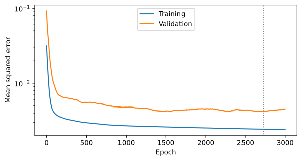

Now the comparison that matters, on the test sample:

with torch.no_grad():
    nn_train = net(torch.tensor(z(train))).numpy().ravel()
    nn_test = net(torch.tensor(z(test))).numpy().ravel()

kitchen_sink = linear_forecasts(predictors)
results = pd.DataFrame({
    "R2 train": [1 - ((train["premium"] - kitchen_sink(train)) ** 2).sum()
                     / ((train["premium"] - benchmark) ** 2).sum(),
                 1 - ((train["premium"] - nn_train) ** 2).sum()
                     / ((train["premium"] - benchmark) ** 2).sum()],
    "R2 test (2000-2025)": [r2_oos(test["premium"], kitchen_sink(test)),
                            r2_oos(test["premium"], nn_test)],
}, index=["Linear, all nine", "Neural network"])
results.round(3)

	R2 train	R2 test (2000-2025)
Linear, all nine	0.056	-0.49
Neural network	0.354	-2.35

Both models explain part of the premium in the sample they were trained on and lose badly to the training-sample average after 2000.

Why the models fail

A model can only learn the relation in the range of data it has seen. The next figure shows the dividend-price ratio with the range it covered in the training sample shaded. After the 1990s it fell far below anything in that range, so every model trained on data up to 1979 had to extrapolate.

fig, ax = plt.subplots(figsize=(7, 3.5))
data["dp"].plot(ax=ax, lw=0.8, label="Log dividend-price ratio")
ax.axhspan(train["dp"].min(), train["dp"].max(), color="0.85", label="Range in training sample")
ax.axvline(pd.Period("2000-01", "M"), color="0.5", ls=":", lw=1)
ax.set_xlabel("")
ax.set_ylabel("")
ax.legend(frameon=False, loc="lower left")
plt.show()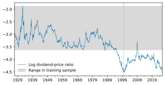

How far outside, in units of the training sample’s standard deviation:

((test[predictors] - mu) / sd).agg(["min", "max"]).round(1)

	dp	ep	bm	tbl	tms	dfy	ntis	svar	infl
min	-4.6	-6.9	-2.6	-1.1	-2.7	-0.7	-3.3	-0.5	-3.4
max	-0.5	0.1	-1.1	1.4	3.0	2.7	0.1	11.4	1.8

A linear model extrapolates along a straight line, and with nine predictors far outside their training range at once, its forecasts swing far more than any plausible expected return. A network extrapolates in ways that depend on its arbitrary weights, so it can do even worse, and how much worse changes with the random seed. Neither problem shows up in the training sample, which is why models are judged on data they have not seen.

Takeaways

• A neural network learns a strong, stable relation from plenty of data with little effort.
• Monthly stock returns offer the opposite: a weak signal, short samples, and predictors whose behavior changes over time. Flexibility then hurts more than it helps.
• Gu et al. (2020) do find gains from machine learning, with tens of thousands of stocks, many characteristics, and models re-estimated as new data arrive. Even then the out-of-sample R^2 is a percent or two a month.

Gu, Shihao, Bryan Kelly, and Dacheng Xiu. 2020. “Empirical Asset Pricing via Machine Learning.” Review of Financial Studies 33 (5): 2223–73. https://doi.org/10.1093/rfs/hhaa009.

Try it

1. Change the seed in torch.manual_seed(0) and train the network again. How much does its test R^2 change?
2. Drop dp, ep and bm, the valuation ratios that drifted furthest, and refit both models. What happens?
3. Re-estimate the linear model every year using all data up to that point, as Welch and Goyal (2008) do, and compare its test R^2 with the fixed model’s.

Welch, Ivo, and Amit Goyal. 2008. “A Comprehensive Look at the Empirical Performance of Equity Premium Prediction.” Review of Financial Studies 21 (4): 1455–508.