Text as Data

This notebook turns the statements of the Federal Open Market Committee (FOMC) into numbers. We collect every policy statement since 2015 from the Federal Reserve’s website and represent each one as a vector, first by counting words and then with embeddings from a small language model. With those vectors we measure how much each statement changed from the previous one, draw a map of the Fed’s communication over a decade, and search the statements by meaning. The notes on language models in finance explain the background.

Packages

requests and BeautifulSoup download and read web pages. sentence-transformers runs a small pretrained language model on your computer; the first time it runs, it downloads the model, about 90 MB.

import re
import time
from pathlib import Path

import matplotlib.pyplot as plt
import numpy as np
import pandas as pd
import requests
from bs4 import BeautifulSoup
from huggingface_hub.utils import logging as hf_logging
from sentence_transformers import SentenceTransformer
from sklearn.feature_extraction.text import CountVectorizer

# Hide the Hugging Face notice about downloading without an account
hf_logging.set_verbosity_error()

DATA = Path("../_data") if Path("../_data").exists() else Path("data")
HEADERS = {"User-Agent": "FIN 4506 course notebook"}

Collecting the statements

The Fed’s calendar pages link each statement, at an address of the form monetaryYYYYMMDDa.htm. The current calendar covers the last few years; older years have a page each.

pages = ["https://www.federalreserve.gov/monetarypolicy/fomccalendars.htm"]
pages += [f"https://www.federalreserve.gov/monetarypolicy/fomchistorical{y}.htm"
          for y in range(2015, pd.Timestamp.today().year)]

dates = set()
for page in pages:
    html = requests.get(page, headers=HEADERS, timeout=30).text
    dates |= set(re.findall(r"/newsevents/pressreleases/monetary(\d{8})a\.htm", html))
dates = sorted(d for d in dates if d >= "20150101")
print(f"{len(dates)} statements, {dates[0]} to {dates[-1]}")

101 statements, 20150128 to 20261028

Each statement page has the date, release information and contact details around the statement itself, which ends where the vote is reported. The function keeps the statement’s paragraphs only. Some of the linked pages are not policy statements: they announce changes to the Fed’s balance sheet operations or to its statement of longer-run goals. A policy statement either reports the vote on “the monetary policy action” or says the Committee “approved the following statement,” so the function also records whether the page is one.

def statement(date):
    url = f"https://www.federalreserve.gov/newsevents/pressreleases/monetary{date}a.htm"
    response = requests.get(url, headers=HEADERS, timeout=30)
    response.encoding = "utf-8"
    article = BeautifulSoup(response.text, "lxml").select_one("#article")
    page = article.get_text(" ", strip=True)
    policy = ("monetary policy action" in page
              or "approved the following statement" in page)
    paragraphs = []
    for p in article.select("p"):
        text = p.get_text(" ", strip=True)
        if text.startswith(("Voting", "For media inquiries",
                            "Implementation Note")):
            break
        if (not text or text.startswith(("For release", "For immediate release"))
                or re.fullmatch(r"[A-Z][a-z]+ \d{1,2}, \d{4}", text)
                or "approved the following statement" in text):
            continue
        paragraphs.append(text)
    return paragraphs, policy

Downloading about a hundred pages takes a minute, so we save the result. The pause between requests is a courtesy to the Fed’s server.

file = DATA / "fomc_releases_2015_2026.parquet"
if not file.exists():
    rows = []
    for date in dates:
        paragraphs, policy = statement(date)
        rows.append({"date": pd.Timestamp(date), "paragraphs": paragraphs, "policy": policy})
        time.sleep(0.5)
    DATA.mkdir(exist_ok=True)
    pd.DataFrame(rows).to_parquet(file)
releases = pd.read_parquet(file)
print("Not policy statements:", list(releases.loc[~releases["policy"], "date"].dt.date))
fomc = releases[releases["policy"]].reset_index(drop=True)
fomc["text"] = fomc["paragraphs"].apply(" ".join)
fomc["words"] = fomc["text"].str.split().str.len()
fomc[["date", "words", "text"]].tail()

Not policy statements: [datetime.date(2019, 10, 11), datetime.date(2020, 3, 31), datetime.date(2020, 8, 27), datetime.date(2025, 8, 22)]

	date	words	text
92	2026-04-29	244	Recent indicators suggest that economic activi...
93	2026-06-17	114	The Committee decided to maintain the target r...
94	2026-07-29	115	The Committee decided to maintain the target r...
95	2026-09-16	114	The Committee decided to raise the target rang...
96	2026-10-28	123	The Committee decided to maintain the target r...

fig, ax = plt.subplots(figsize=(7, 3))
ax.plot(fomc["date"], fomc["words"], "o", ms=3)
ax.set_ylabel("Words")
ax.set_title("Length of FOMC statements")
plt.show()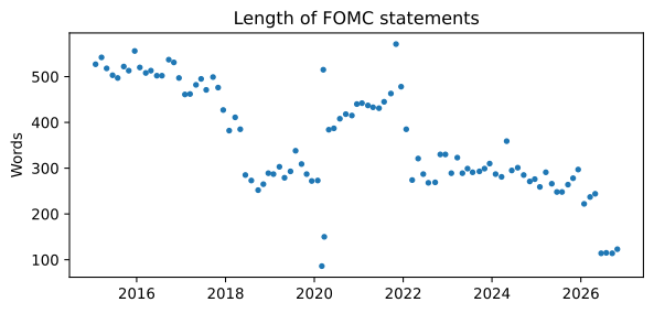

How much did the statement change? Counting words

A first measure of change compares each statement’s word counts with the previous statement’s. CountVectorizer builds the bag-of-words vectors, one entry per word, and the cosine similarity of consecutive vectors measures how much the wording stayed the same. We define the change as one minus the similarity.

counts = CountVectorizer().fit_transform(fomc["text"]).toarray().astype(float)

def change_from_previous(vectors):
    unit = vectors / np.linalg.norm(vectors, axis=1, keepdims=True)
    similarity = (unit[1:] * unit[:-1]).sum(axis=1)
    return np.r_[np.nan, 1 - similarity]

fomc["change_words"] = change_from_previous(counts)

How much did the statement change? Embeddings

The model all-MiniLM-L6-v2 maps a piece of text to a vector of 384 numbers, so that texts with similar meanings get vectors that point in similar directions. It reads at most about 256 tokens at a time and would cut longer texts short, so we embed each paragraph separately and average the paragraphs’ vectors into one vector per statement.

model = SentenceTransformer("all-MiniLM-L6-v2")

def embed_statement(paragraphs):
    vectors = model.encode(list(paragraphs), normalize_embeddings=True, show_progress_bar=False)
    return vectors.mean(axis=0)

embeddings = np.vstack([embed_statement(p) for p in fomc["paragraphs"]])
fomc["change_meaning"] = change_from_previous(embeddings)
embeddings.shape

(97, 384)

The two measures agree on the big changes and disagree on smaller ones: a statement can reword many sentences without changing its message, or change its message with a few words.

fig, ax = plt.subplots(figsize=(6, 4))
ax.scatter(fomc["change_words"], fomc["change_meaning"], s=12)
for _, row in fomc.nlargest(3, "change_meaning").iterrows():
    ax.annotate(f"{row['date']:%b %d, %Y}", (row["change_words"], row["change_meaning"]),
                xytext=(4, 2), textcoords="offset points", fontsize=8)
ax.margins(x=0.15)
ax.set_xlabel("Change in wording (word counts)")
ax.set_ylabel("Change in meaning (embeddings)")
plt.show()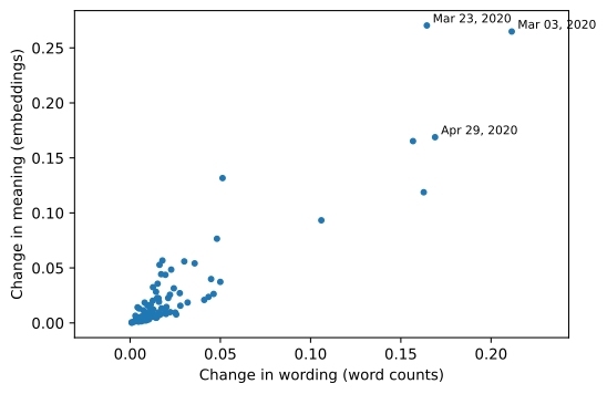

Change in meaning over time

How do the large changes line up with what the Fed did? The upper bound of the federal funds target range comes from FRED, series DFEDTARU.

url = "https://fred.stlouisfed.org/graph/fredgraph.csv?id=DFEDTARU"
target = pd.read_csv(url, parse_dates=["observation_date"],
                     index_col="observation_date")["DFEDTARU"].dropna()

before = fomc["date"].map(lambda t: target.asof(t - pd.Timedelta(days=1)))
after = fomc["date"].map(lambda t: target.asof(t + pd.Timedelta(days=1)))
fomc["action"] = np.select([after > before, after < before], ["hike", "cut"], "hold")
fomc["action"].value_counts()

action
hold    65
hike    21
cut     11
Name: count, dtype: int64

fig, (ax1, ax2) = plt.subplots(2, 1, figsize=(8, 5), sharex=True,
                               gridspec_kw={"height_ratios": [3, 2]})
ax1.vlines(fomc["date"], 0, fomc["change_meaning"], lw=1.5)
labeled = []
for _, row in fomc.nlargest(7, "change_meaning").iterrows():
    # One label per cluster of large changes
    if all(abs((row["date"] - d).days) > 90 for d in labeled):
        labeled.append(row["date"])
        ax1.annotate(f"{row['date']:%b %Y}", (row["date"], row["change_meaning"]),
                     xytext=(3, 0), textcoords="offset points", fontsize=8)
ax1.set_ylabel("Change in meaning")
ax2.step(target.loc["2015":].index, target.loc["2015":], where="post")
ax2.set_ylabel("Fed funds target (%)")
plt.show()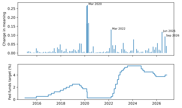

The largest changes come when policy turned abruptly: the emergency cuts of March 2020 and the statements that followed, the first hike of the 2022 cycle, in March 2022, and the first hike after the cuts of 2024 and 2025, in September 2026. Two cautions keep this from being a rule. Not every turning point shows up: the first cut of September 2024 barely changed the statement’s meaning, although it was a turning point in policy. And not every large change is about policy: in June 2026 the Fed adopted a new, much shorter format for its statements, which changed the text a great deal without changing the policy.

A map of Fed communication

An embedding has 384 numbers, too many to look at. Principal components find the two directions along which the statements differ most, and projecting each statement onto them gives a map in two dimensions. Nothing in the calculation knows the dates.

centered = embeddings - embeddings.mean(axis=0)
_, singular_values, directions = np.linalg.svd(centered, full_matrices=False)
fomc[["pc1", "pc2"]] = centered @ directions[:2].T
share = singular_values[:2] ** 2 / (singular_values**2).sum()
print(f"Share of the variation along the two directions: {share.round(2)}")

Share of the variation along the two directions: [0.33 0.18]

periods = pd.cut(fomc["date"].dt.year, [2014, 2019, 2021, 2023, 2026],
                 labels=["2015-2019", "2020-2021", "2022-2023", "2024-2026"])
fig, ax = plt.subplots(figsize=(6.5, 4.5))
for period, group in fomc.groupby(periods, observed=True):
    ax.scatter(group["pc1"], group["pc2"], s=18, label=period)
ax.set_xlabel("First principal component")
ax.set_ylabel("Second principal component")
ax.legend(frameon=False)
plt.show()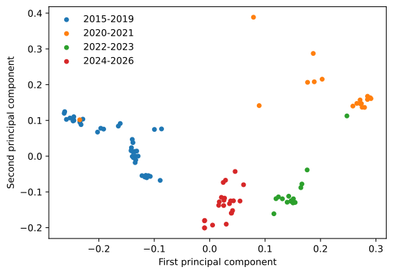

The statements sort themselves into the Fed’s recent history: the slow normalization of 2015 to 2019, the pandemic years of zero rates, the rapid hikes of 2022 and 2023, and the period since. Statements written in the same circumstances use different sentences but carry similar meanings, and the embeddings place them together.

Does meaning also track what the Fed did at each meeting? For each statement, find the most similar other statement, skipping the two meetings before and after it, which are similar simply because they are close in time, and check whether the Fed took the same action, hike, hold or cut, at both meetings.

unit = embeddings / np.linalg.norm(embeddings, axis=1, keepdims=True)
similarity = unit @ unit.T
n = len(fomc)
for i in range(n):
    similarity[i, max(0, i - 2):i + 3] = -np.inf
nearest = similarity.argmax(axis=1)
same = (fomc["action"].to_numpy() == fomc["action"].to_numpy()[nearest]).mean()
chance = (fomc["action"].value_counts(normalize=True) ** 2).sum()
print(f"Same action as the nearest statement: {same:.0%}   (by chance: {chance:.0%})")

Same action as the nearest statement: 67%   (by chance: 51%)

The nearest statement in meaning shares the action more often than chance would give. Part of this is still the eras: skipping two meetings on each side leaves neighbors from the same hiking or holding cycle, so the test does not separate what the Fed said from when it said it.

Search by meaning

Embeddings also make search by meaning possible. Which statement is closest to a sentence we write ourselves?

query = "Inflation is far too high and the Committee will raise rates aggressively."
q = model.encode([query], normalize_embeddings=True)[0]
fomc.assign(similarity=unit @ q).nlargest(3, "similarity")[["date", "action", "similarity"]]

	date	action	similarity
63	2022-09-21	hike	0.707931
62	2022-07-27	hike	0.707741
64	2022-11-02	hike	0.701451

What embeddings can and cannot tell us

An embedding from a small general-purpose model captures what a text is about and how it is framed, well enough to sort a decade of statements into eras and to find the statements that match a description. It does not know which way a statement points for markets, or what markets expected before it came out. A statement can change a great deal in meaning because the economy changed, while telling investors nothing they did not already know.

Try it

1. Change the query in the search, for example to a sentence about the labor market or about financial stability, and read the statements it finds.
2. Find the two consecutive statements whose meaning changed least, read them, and explain what changed in their wording.
3. Do yields move with the statements? Collect the daily change in the 2-year Treasury yield (FRED series DGS2) on each statement day and plot it against the change in meaning. Before drawing conclusions, consider what else happens that day. On June 15, 2022 and December 13, 2023, the 2-year yield fell by more than 20 basis points although the statements’ meaning changed little: at those meetings the Fed also released its economic projections, and, as at every meeting since 2019, the chair held a press conference. Research on central bank communication, such as Gürkaynak et al. (2005), uses yield changes within minutes of the release for this reason.

Gürkaynak, Refet S., Brian Sack, and Eric T. Swanson. 2005. “Do Actions Speak Louder Than Words? The Response of Asset Prices to Monetary Policy Actions and Statements.” International Journal of Central Banking 1 (1): 55–93. https://www.ijcb.org/journal/v1n1/do-actions-speak-louder-words-response-asset-prices-monetary-policy-actions-and.