import os
import platform
from pathlib import Path

import matplotlib.pyplot as plt
import numpy as np
import pandas as pd
import statsmodels.formula.api as smf
import yfinance as yfPython, Data and WRDS
This notebook covers the data work the rest of the course builds on: loading data from a free public source and from WRDS, computing returns and their risk, drawing a figure, and running a regression. You used Python or R in the first half of the course; here the point is less the syntax, which Claude can write for you, than knowing where the data come from and what each step does to them.
Run it in the course environment you set up for your class log. The WRDS part needs your WRDS account.
Packages
Data from a public source: FRED
The Federal Reserve Bank of St. Louis publishes thousands of economic series on FRED. Any series downloads as a CSV file from a URL that contains its ID, with no account or key. DGS10 is the 10-year Treasury yield, in percent.
url = "https://fred.stlouisfed.org/graph/fredgraph.csv?id=DGS10"
dgs10 = pd.read_csv(url, parse_dates=["observation_date"], index_col="observation_date")
dgs10.tail()| DGS10 | |
|---|---|
| observation_date | |
| 2026-11-03 | 4.95 |
| 2026-11-04 | 4.90 |
| 2026-11-05 | 4.84 |
| 2026-11-06 | 4.86 |
| 2026-11-09 | 4.88 |
The file has one row per business day. Days when markets were closed are missing values, which dropna() removes.
fig, ax = plt.subplots(figsize=(8, 3.5))
dgs10["DGS10"].dropna().plot(ax=ax, lw=0.8)
ax.set_xlabel("")
ax.set_ylabel("Percent")
ax.set_title("10-year Treasury yield")
plt.show()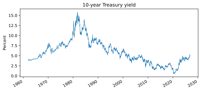
Data from WRDS
WRDS gives researchers and students access to the databases used in most academic finance: CRSP for stock prices and returns, Compustat for accounting data, OptionMetrics for options, and many more. WRDS keeps them in a PostgreSQL database, so we query them with SQL, the standard language for databases, through a small Python package called psycopg.
Your password, once
The connection reads your WRDS username and password from a file called pgpass, which only you can read. Run the next cell once on your computer: it asks for your password and writes the file. On WRDS’s first connection you may also be asked to approve the login with Duo.
from getpass import getpass

username = input("WRDS username: ")
password = getpass("WRDS password: ")
line = f"wrds-pgdata.wharton.upenn.edu:9737:wrds:{username}:{password}\n"

if platform.system() == "Windows":
    pgpass = Path(os.environ["APPDATA"]) / "postgresql" / "pgpass.conf"
else:
    pgpass = Path.home() / ".pgpass"
pgpass.parent.mkdir(exist_ok=True)
pgpass.write_text(line)
pgpass.chmod(0o600)
print("Saved to", pgpass)
A function that runs a query
The function below connects to WRDS, runs a query, and returns the result as a pandas DataFrame. It also saves the result as a file in a data folder, so that running the notebook again reads the file instead of querying WRDS. Delete the file to download the data again.
import psycopg
from psycopg.types.numeric import FloatLoader

def wrds_username():
    """Your WRDS username, read from the pgpass file."""
    if platform.system() == "Windows":
        pgpass = Path(os.environ["APPDATA"]) / "postgresql" / "pgpass.conf"
    else:
        pgpass = Path.home() / ".pgpass"
    for line in pgpass.read_text().splitlines():
        if line.startswith("wrds-pgdata"):
            return line.split(":")[3]

DATA = Path("../_data") if Path("../_data").exists() else Path("data")

def wrds_query(name, sql):
    """Run a SQL query on WRDS and cache the result in DATA/<name>.parquet."""
    file = DATA / f"{name}.parquet"
    if not file.exists():
        with psycopg.connect(host="wrds-pgdata.wharton.upenn.edu", port=9737,
                             dbname="wrds", user=wrds_username(),
                             sslmode="require") as conn:
            # Return SQL numbers as floats rather than Python Decimals
            conn.adapters.register_loader("numeric", FloatLoader)
            cur = conn.execute(sql)
            df = pd.DataFrame(cur.fetchall(), columns=[c.name for c in cur.description])
        DATA.mkdir(exist_ok=True)
        df.to_parquet(file)
    return pd.read_parquet(file)
Monthly stock returns from CRSP
CRSP identifies each stock by a permanent number, permno, because tickers change and are reused. The monthly stock file is crsp.msf_v2. Its column mthret is the monthly return including dividends, and mthcaldt is the last trading day of the month. We take three large stocks from 2015 to 2025.
stocks = wrds_query("crsp_msf_aapl_msft_jpm_2015_2025", """
    SELECT permno, ticker, mthcaldt AS date, mthret AS ret
    FROM crsp.msf_v2
    WHERE permno IN (14593, 10107, 47896)
      AND mthcaldt BETWEEN '2015-01-01' AND '2025-12-31'
""")
stocks.head()| permno | ticker | date | ret | |
|---|---|---|---|---|
| 0 | 10107 | MSFT | 2015-01-30 | -0.130248 |
| 1 | 10107 | MSFT | 2015-02-27 | 0.093117 |
| 2 | 10107 | MSFT | 2015-03-31 | -0.072862 |
| 3 | 10107 | MSFT | 2015-04-30 | 0.196409 |
| 4 | 10107 | MSFT | 2015-05-29 | -0.030319 |
The data come in long format: one row per stock and month. For most calculations a wide table, with one column per stock, is easier. pivot does the reshaping.
rets = stocks.pivot(index="date", columns="ticker", values="ret")
rets.index = pd.to_datetime(rets.index).to_period("M")
rets.tail()| ticker | AAPL | JPM | MSFT |
|---|---|---|---|
| date | |||
| 2025-08 | 0.119650 | 0.017486 | -0.048690 |
| 2025-09 | 0.096881 | 0.046480 | 0.022223 |
| 2025-10 | 0.061815 | -0.008879 | -0.000270 |
| 2025-11 | 0.032360 | 0.006300 | -0.048018 |
| 2025-12 | -0.025067 | 0.029194 | -0.017053 |
We also need the return on the market and the risk-free rate. The CRSP value-weighted index, which holds every stock in proportion to its market value, is index number 1000200 in crsp.indmthseriesdata. The one-month Treasury bill rate is in the Fama-French factors on WRDS, in ff.factors_monthly.
mkt = wrds_query("crsp_vw_2015_2025", """
    SELECT mthcaldt AS date, mthtotret AS mkt
    FROM crsp.indmthseriesdata
    WHERE indno = 1000200 AND mthcaldt BETWEEN '2015-01-01' AND '2025-12-31'
""")
rf = wrds_query("ff_rf_2015_2025", """
    SELECT date, rf
    FROM ff.factors_monthly
    WHERE date BETWEEN '2015-01-01' AND '2025-12-31'
""")
mkt.index = pd.to_datetime(mkt.pop("date")).dt.to_period("M")
rf.index = pd.to_datetime(rf.pop("date")).dt.to_period("M")

df = rets.join(mkt).join(rf).dropna()
df.tail()| AAPL | JPM | MSFT | mkt | rf | |
|---|---|---|---|---|---|
| date | |||||
| 2025-08 | 0.119650 | 0.017486 | -0.048690 | 0.024123 | 0.0038 |
| 2025-09 | 0.096881 | 0.046480 | 0.022223 | 0.035626 | 0.0033 |
| 2025-10 | 0.061815 | -0.008879 | -0.000270 | 0.019284 | 0.0037 |
| 2025-11 | 0.032360 | 0.006300 | -0.048018 | 0.001997 | 0.0030 |
| 2025-12 | -0.025067 | 0.029194 | -0.017053 | 0.001297 | 0.0034 |
Joining on monthly periods matters here: CRSP dates a month by its last trading day and the Fama-French file by its first day, so the raw dates never match.
Returns and risk
The average monthly return and its standard deviation, the volatility, describe each asset. Multiplying the average by 12 and the standard deviation by \sqrt{12} puts them in annual terms, which assumes that monthly returns are independent over time.
assets = ["AAPL", "MSFT", "JPM", "mkt"]
summary = pd.DataFrame({
    "mean (annual)": df[assets].mean() * 12,
    "volatility (annual)": df[assets].std() * np.sqrt(12),
})
summary.round(3)| mean (annual) | volatility (annual) | |
|---|---|---|
| AAPL | 0.257 | 0.271 |
| MSFT | 0.253 | 0.220 |
| JPM | 0.206 | 0.241 |
| mkt | 0.125 | 0.152 |
The growth of one dollar invested at the start shows the same returns as a path. Compounding monthly returns gives the value of the investment at the end of each month.
growth = (1 + df[assets]).cumprod()

fig, ax = plt.subplots(figsize=(8, 4))
growth.rename(columns={"mkt": "Market"}).plot(ax=ax, logy=True)
ax.set_xlabel("")
ax.set_ylabel("Value of $1 (log scale)")
ax.set_title("Growth of $1, 2015 to 2025")
plt.show()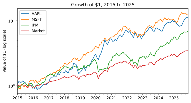
A first regression
How much does a stock move with the market? Regressing the stock’s excess return, its return above the risk-free rate, on the market’s excess return gives the stock’s beta, the slope of the line.
df["aapl_ex"] = df["AAPL"] - df["rf"]
df["mkt_ex"] = df["mkt"] - df["rf"]

res = smf.ols("aapl_ex ~ mkt_ex", data=df).fit()
print(res.summary().tables[1])
==============================================================================
coef std err t P>|t| [0.025 0.975]
------------------------------------------------------------------------------
Intercept 0.0098 0.005 1.815 0.072 -0.001 0.020
mkt_ex 1.1389 0.121 9.425 0.000 0.900 1.378
==============================================================================The slope on mkt_ex is Apple’s beta and the intercept is its alpha, the average excess return the market does not explain. The p-value tests whether each coefficient is zero. To test whether the beta equals one, the beta of the market itself, use an F-test:
print(f"beta: {res.params['mkt_ex']:.2f}")
print(f"p-value (H0: beta = 1): {float(res.f_test('mkt_ex = 1').pvalue):.3f}")
print(f"R-squared: {res.rsquared:.2f}")
beta: 1.14
p-value (H0: beta = 1): 0.252
R-squared: 0.41Crypto from Yahoo Finance
WRDS does not cover cryptocurrencies, but Yahoo Finance does. The yfinance package downloads Yahoo’s prices. It is not an official interface, so it can stop working without notice; save what you download.
btc = yf.download("BTC-USD", start="2015-01-01", end="2026-01-01",
                  auto_adjust=True, progress=False)["Close"]
btc_ret = btc["BTC-USD"].resample("ME").last().pct_change().dropna()
btc_ret.index = btc_ret.index.to_period("M")

both = pd.concat([btc_ret.rename("BTC"), df["mkt"]], axis=1).dropna()
print(f"Bitcoin annual volatility: {both['BTC'].std() * np.sqrt(12):.2f}")
print(f"Market annual volatility:  {both['mkt'].std() * np.sqrt(12):.2f}")
print(f"Correlation of monthly returns: {both.corr().iloc[0, 1]:.2f}")
Bitcoin annual volatility: 0.72
Market annual volatility: 0.15
Correlation of monthly returns: 0.34Bitcoin trades every day of the week, so its month ends on the last calendar day, while the stock market’s ends on the last trading day. With monthly returns the difference is small; with daily returns you would have to align the two calendars.
Try it
- Add Nvidia (
permno86580) to the stock query and compute its beta. Remember to give the cached file a new name, or delete the old one. - Download
DGS2, the 2-year Treasury yield, from FRED and plot the difference between the 10-year and the 2-year yield. - Compute the correlation between Bitcoin and the market separately for 2015 to 2019 and for 2020 to 2025. What changed?