Pricing Options with Neural Networks

This notebook trains a neural network to predict the implied volatilities of options on the S&P 500 index, using prices from OptionMetrics on WRDS. We train on 2024, choose when to stop on early 2025, and test on May to August 2025, months the network has not seen. Two benchmarks keep it honest: Black-Scholes with a single volatility, and a simple regression that can bend into a smile. The notes on neural networks and option pricing explain the background.

Packages and the WRDS function

The wrds_query function is the one from the notebook on Python, data and WRDS: it runs a SQL query on WRDS and saves the result.

import os
import platform
from pathlib import Path

import matplotlib.pyplot as plt
import numpy as np
import pandas as pd
import psycopg
import torch
import torch.nn as nn
from psycopg.types.numeric import FloatLoader

torch.manual_seed(0)

def wrds_username():
    if platform.system() == "Windows":
        pgpass = Path(os.environ["APPDATA"]) / "postgresql" / "pgpass.conf"
    else:
        pgpass = Path.home() / ".pgpass"
    for line in pgpass.read_text().splitlines():
        if line.startswith("wrds-pgdata"):
            return line.split(":")[3]
    raise RuntimeError(f"No WRDS line in {pgpass}; run the password cell in the WRDS notebook first.")

DATA = Path("../_data") if Path("../_data").exists() else Path("data")

def wrds_query(name, sql):
    file = DATA / f"{name}.parquet"
    if not file.exists():
        with psycopg.connect(host="wrds-pgdata.wharton.upenn.edu", port=9737,
                             dbname="wrds", user=wrds_username(),
                             sslmode="require") as conn:
            conn.adapters.register_loader("numeric", FloatLoader)
            cur = conn.execute(sql)
            df = pd.DataFrame(cur.fetchall(), columns=[c.name for c in cur.description])
        DATA.mkdir(exist_ok=True)
        df.to_parquet(file)
    return pd.read_parquet(file)

The data

OptionMetrics stores one table of option prices per year, optionm.opprcd2024, optionm.opprcd2025 and so on, and one table of underlying prices, optionm.secprd2024 and so on. The S&P 500 index has security ID 108105. We keep:

• Wednesdays only, which is plenty of data and avoids weekend effects;
• the standard monthly contracts, whose symbol starts with SPX followed by a space (the weekly contracts start with SPXW);
• options with a positive bid and an implied volatility;
• maturities between 7 days and one year, and strikes between 80% and 120% of the index;
• out-of-the-money options only, puts below the index level and calls above it, which trade most.

Strikes are stored multiplied by 1,000.

query = """
    SELECT o.date, o.exdate, o.cp_flag, o.strike_price / 1000.0 AS strike,
           o.best_bid AS bid, o.best_offer AS ask, o.impl_volatility AS iv,
           s.close AS spot
    FROM optionm.opprcd{year} o
    JOIN optionm.secprd{year} s ON s.secid = o.secid AND s.date = o.date
    WHERE o.secid = 108105
      AND EXTRACT(DOW FROM o.date) = 3
      AND o.date <= '2025-08-31'
      AND o.symbol LIKE 'SPX %'
      AND o.best_bid > 0 AND o.impl_volatility IS NOT NULL
      AND o.exdate - o.date BETWEEN 7 AND 365
      AND o.strike_price / 1000.0 / s.close BETWEEN 0.8 AND 1.2
      AND ((o.cp_flag = 'P' AND o.strike_price / 1000.0 < s.close)
        OR (o.cp_flag = 'C' AND o.strike_price / 1000.0 >= s.close))
"""
options = pd.concat([wrds_query(f"optionm_spx_wed_{y}", query.format(year=y))
                     for y in (2024, 2025)], ignore_index=True)
options["date"] = pd.to_datetime(options["date"])
options["exdate"] = pd.to_datetime(options["exdate"])
print(f"{len(options):,} options on {options['date'].nunique()} days, "
      f"{options['date'].min():%B %d, %Y} to {options['date'].max():%B %d, %Y}")

155,554 options on 84 days, January 03, 2024 to August 27, 2025

The VIX, a market-wide measure of expected volatility, comes from FRED.

vix = pd.read_csv("https://fred.stlouisfed.org/graph/fredgraph.csv?id=VIXCLS",
                  parse_dates=["observation_date"], index_col="observation_date")["VIXCLS"]
options = options.join(vix.rename("vix"), on="date").dropna()

The model’s inputs are the log of moneyness, \ln(K/S), the time to maturity in years, and the VIX as a decimal. The output is the implied volatility.

options["log_m"] = np.log(options["strike"] / options["spot"])
options["T"] = (options["exdate"] - options["date"]).dt.days / 365
options["vix_dec"] = options["vix"] / 100
features = ["log_m", "T", "vix_dec"]

The skew changes with the market. On a calm day and on a day during the sell-off of April 2025, the three-month skew looks like this. The small jump at a log moneyness of zero is where the data switch from puts to calls.

fig, ax = plt.subplots(figsize=(7, 3.5))
for day in [options["date"].min(), pd.Timestamp("2025-04-09")]:
    d = options[options["date"] == day]
    T = d["T"].unique()[np.argmin(np.abs(d["T"].unique() - 0.25))]
    d = d[d["T"] == T].sort_values("log_m")
    ax.plot(d["log_m"], 100 * d["iv"], label=f"{day:%B %d, %Y} (VIX {d['vix'].iloc[0]:.0f})")
ax.set_xlabel("Log moneyness ln(K/S)")
ax.set_ylabel("Implied volatility (%)")
ax.legend(frameon=False)
plt.show()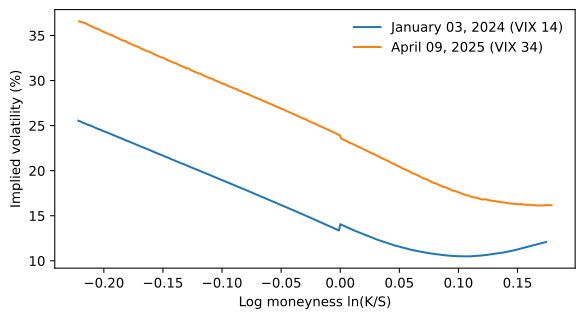

Training, validation and test samples

The split is by time, as it would be in practice: the model is trained on the past and used on the future.

train = options[options["date"] < "2025-01-01"]
valid = options[(options["date"] >= "2025-01-01") & (options["date"] < "2025-05-01")]
test = options[options["date"] >= "2025-05-01"]
print(f"train {len(train):,}   validation {len(valid):,}   test {len(test):,}")

train 87,457   validation 33,564   test 34,533

We measure errors as the mean absolute difference between predicted and actual implied volatility, in volatility points: an error of 1.0 means, for example, predicting 16% when the market says 15%.

mae = lambda actual, predicted: 100 * np.mean(np.abs(actual - predicted))

Two benchmarks

The first benchmark is Black-Scholes with one volatility for every option: the VIX. It cannot produce a skew.

flat = {name: df["vix_dec"].to_numpy() for name, df in
        [("train", train), ("valid", valid), ("test", test)]}

The second is a linear regression with squared and interaction terms, which lets the curve bend with moneyness and shift with maturity and the VIX. It is the kind of parametric smile a practitioner might fit by hand.

def design(df):
    x, T, v = df["log_m"].to_numpy(), df["T"].to_numpy(), df["vix_dec"].to_numpy()
    return np.c_[np.ones(len(df)), x, x**2, T, np.sqrt(T), x * T, v, x * v]

beta = np.linalg.lstsq(design(train), train["iv"], rcond=None)[0]
quad = {name: design(df) @ beta for name, df in
        [("train", train), ("valid", valid), ("test", test)]}

The neural network

The inputs are standardized with the training sample’s means and standard deviations. The network has two hidden layers of 32 units, and we keep the weights with the lowest validation loss.

mu, sd = train[features].mean(), train[features].std()
to_x = lambda df: torch.tensor(((df[features] - mu) / sd).to_numpy(), dtype=torch.float32)
to_y = lambda df: torch.tensor(df[["iv"]].to_numpy(), dtype=torch.float32)

net = nn.Sequential(
    nn.Linear(3, 32), nn.ReLU(),
    nn.Linear(32, 32), nn.ReLU(),
    nn.Linear(32, 1),
)
opt = torch.optim.Adam(net.parameters(), lr=0.003)

X_train, y_train = to_x(train), to_y(train)
X_valid, y_valid = to_x(valid), to_y(valid)
history, best_loss = [], np.inf
for epoch in range(1500):
    opt.zero_grad()
    loss = ((net(X_train) - y_train) ** 2).mean()
    loss.backward()
    opt.step()
    with torch.no_grad():
        valid_loss = ((net(X_valid) - y_valid) ** 2).mean().item()
    history.append((loss.item(), valid_loss))
    if valid_loss < best_loss:
        best_loss, best_epoch = valid_loss, epoch
        best_weights = {k: v.clone() for k, v in net.state_dict().items()}
net.load_state_dict(best_weights)
print(f"Lowest validation loss at epoch {best_epoch}")

Lowest validation loss at epoch 849

fig, ax = plt.subplots(figsize=(7, 3.5))
pd.DataFrame(history, columns=["Training", "Validation"]).plot(ax=ax)
ax.axvline(best_epoch, color="0.5", ls=":", lw=1)
ax.set_yscale("log")
ax.set_xlabel("Epoch")
ax.set_ylabel("Mean squared error")
plt.show()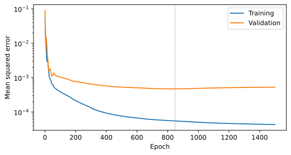

Results

with torch.no_grad():
    nn_pred = {name: net(to_x(df)).numpy().ravel() for name, df in
               [("train", train), ("valid", valid), ("test", test)]}

samples = {"train": train, "valid": valid, "test": test}
results = pd.DataFrame({
    model: {name: mae(samples[name]["iv"], pred[name]) for name in samples}
    for model, pred in [("Black-Scholes, one volatility", flat),
                        ("Quadratic regression", quad),
                        ("Neural network", nn_pred)]
}).T
results.columns = ["Train (2024)", "Validation (Jan-Apr 2025)", "Test (May-Aug 2025)"]
results.round(2)

	Train (2024)	Validation (Jan-Apr 2025)	Test (May-Aug 2025)
Black-Scholes, one volatility	4.79	5.48	5.08
Quadratic regression	1.61	2.10	1.87
Neural network	0.53	1.42	1.26

Where do the errors come from? Splitting the test sample by moneyness:

bins = pd.cut(test["log_m"], [-0.23, -0.15, -0.08, -0.02, 0.02, 0.19],
              labels=["Deep OTM puts", "OTM puts", "Near-money puts",
                      "At the money", "OTM calls"])
by_m = pd.DataFrame({
    "Black-Scholes, one volatility": np.abs(test["iv"] - flat["test"]),
    "Quadratic regression": np.abs(test["iv"] - quad["test"]),
    "Neural network": np.abs(test["iv"] - nn_pred["test"]),
}).mul(100).groupby(bins, observed=True).mean()

fig, ax = plt.subplots(figsize=(8, 3.5))
by_m.plot.bar(ax=ax, rot=0)
ax.set_xlabel("")
ax.set_ylabel("Mean absolute error (vol points)")
ax.legend(frameon=False)
plt.show()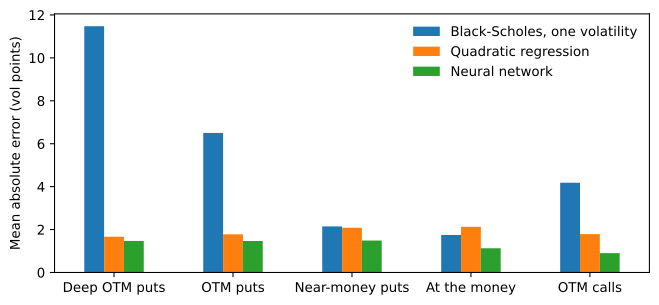

And on one day in the test sample, the three-month skew as the market priced it and as each model predicted it:

day = test["date"].max()
d = test[test["date"] == day]
T = d["T"].unique()[np.argmin(np.abs(d["T"].unique() - 0.25))]
mask = (test["date"] == day) & (test["T"] == T)
d = test[mask].assign(flat=flat["test"][mask.to_numpy()],
                      quad=quad["test"][mask.to_numpy()],
                      net=nn_pred["test"][mask.to_numpy()]).sort_values("log_m")

fig, ax = plt.subplots(figsize=(7, 3.5))
ax.scatter(d["log_m"], 100 * d["iv"], s=8, color="0.4", label="Market")
ax.plot(d["log_m"], 100 * d["flat"], label="Black-Scholes, one volatility")
ax.plot(d["log_m"], 100 * d["quad"], label="Quadratic regression")
ax.plot(d["log_m"], 100 * d["net"], label="Neural network")
ax.set_title(f"{day:%B %d, %Y}, {round(T * 365)} days to maturity")
ax.set_xlabel("Log moneyness ln(K/S)")
ax.set_ylabel("Implied volatility (%)")
ax.legend(frameon=False)
plt.show()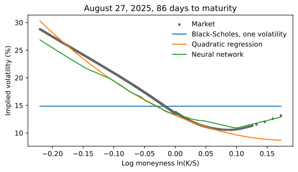

What we learned

• A single volatility misses the skew, so its errors are large and largest for the low strikes where the skew is steepest.
• A regression with a few curved terms captures most of the skew, though near the money it does no better than a single volatility. A benchmark like this is what a network has to beat to be worth its complexity.
• The network beats both on months it has not seen. This is a fit of the shape of each day’s volatility surface given its level, not a forecast: the VIX is computed from the same day’s S&P 500 options. Here, unlike in predicting the stock market, the signal is strong, the data are plentiful, and the test inputs lie mostly within the range of the training data.
• Its training error is still well below its test error: some of what it learned from 2024 did not carry over to 2025.

Try it

1. Add a fourth input, such as the S&P 500’s return over the previous month, and see whether the test error falls.
2. Compute the network’s errors date by date over the validation sample. How did it do during the sell-off in early April 2025, when the VIX rose above anything in 2024?
3. Convert the network’s implied volatilities for one maturity into call prices with the Black-Scholes formula, and check whether the prices are decreasing and convex in the strike.