Liquidation Cascades

This notebook simulates a lending protocol in a falling market. Two thousand borrowers have deposited ETH and borrowed dollar stablecoins against it. When the price of ETH falls, the loans whose health factor drops below one are liquidated, the liquidators sell the ETH they receive, and the sales push the price down further, which can trigger more liquidations. We measure how much a first price drop is amplified, and how that depends on how deep the market is and on how large the first drop is. The notes on lending protocols and liquidations explain the background.

Packages

import matplotlib.pyplot as plt
import numpy as np
import pandas as pd

rng = np.random.default_rng(0)

The loans

Each borrower deposits some ETH, with amounts that vary a lot from borrower to borrower, and borrows USDC up to a chosen health factor between 1.05 and 2: some borrow cautiously, others close to the limit. ETH has a liquidation threshold of 0.80.

P0 = 3_000          # price of ETH at the start
THRESHOLD = 0.80    # liquidation threshold of ETH
CLOSE_FACTOR = 0.5  # share of the debt a liquidator can repay at once
BONUS = 0.05        # liquidation bonus

n = 2_000
collateral = rng.lognormal(np.log(10), 0.8, n)       # ETH deposited
health = rng.uniform(1.05, 2.0, n)                   # health factor chosen at the start
debt = collateral * P0 * THRESHOLD / health          # USDC borrowed
liq_price = debt / (collateral * THRESHOLD)          # price at which the loan becomes liquidatable

print(f"Collateral: {collateral.sum():,.0f} ETH, worth ${collateral.sum() * P0 / 1e6:,.0f} million")
print(f"Debt: ${debt.sum() / 1e6:,.0f} million")

Collateral: 26,782 ETH, worth $80 million
Debt: $44 million

fig, ax = plt.subplots(figsize=(7, 3.2))
ax.hist(liq_price, bins=np.linspace(1500, 3000, 61), color="0.6")
ax.axvline(P0, color="0.2", lw=1)
ax.set_xlabel("Liquidation price of each loan")
ax.set_ylabel("Number of loans")
plt.show()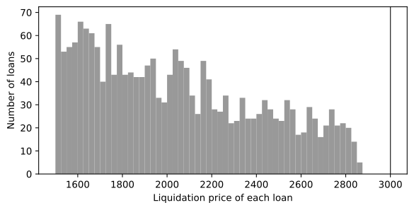

The market

Liquidators sell the ETH they receive. We represent everywhere they can sell it within minutes by a single constant-product pool, like the one in the notebook on automated market makers, whose price the protocol also uses as its oracle. The pool’s depth, the dollar value of its reserves, stands for how much selling the market can absorb: the deeper it is, the less each sale moves the price.

class Pool:
    def __init__(self, depth):
        self.eth = depth / 2 / P0
        self.usdc = depth / 2
        self.k = self.eth * self.usdc

    @property
    def price(self):
        return self.usdc / self.eth

    def sell_eth(self, amount):
        self.eth += amount
        self.usdc = self.k / self.eth

    def drop_price(self, fraction):
        """An outside seller pushes the price down by the given fraction."""
        self.eth = np.sqrt(self.k / (self.price * (1 - fraction)))
        self.usdc = self.k / self.eth

A cascade

Starting from a first drop in the price, we repeat the same round until no loan is left to liquidate. In each round, every loan with a health factor below one is liquidated: the liquidator repays half its debt, receives ETH worth the repaid debt plus the 5% bonus, and sells that ETH into the pool.

def cascade(depth, first_drop, max_rounds=500):
    pool = Pool(depth)
    pool.drop_price(first_drop)
    coll, dbt = collateral.copy(), debt.copy()
    prices, liquidated = [pool.price], 0.0
    for _ in range(max_rounds):
        p = pool.price
        hf = np.full(n, np.inf)
        open_loans = dbt > 1e-6
        hf[open_loans] = coll[open_loans] * p * THRESHOLD / dbt[open_loans]
        hit = (hf < 1) & (coll > 1e-9)
        if not hit.any():
            break
        seized = np.minimum(CLOSE_FACTOR * dbt[hit] * (1 + BONUS) / p, coll[hit])
        dbt[hit] -= seized * p / (1 + BONUS)
        coll[hit] -= seized
        liquidated += seized.sum() * p
        pool.sell_eth(seized.sum())
        prices.append(pool.price)
    bad_debt = dbt[(coll <= 1e-9) & (dbt > 1e-6)].sum()
    return {"prices": prices, "final_price": prices[-1], "rounds": len(prices) - 1,
            "liquidated": liquidated, "bad_debt": bad_debt}

How market depth changes the cascade

A first drop of 10%, in markets of different depths:

rows = []
for depth in [200e6, 250e6, 300e6, 500e6, 1_000e6]:
    r = cascade(depth, 0.10)
    rows.append({"depth ($ millions)": depth / 1e6,
                 "final change in price": r["final_price"] / P0 - 1,
                 "rounds": r["rounds"],
                 "liquidated ($ millions)": r["liquidated"] / 1e6,
                 "bad debt ($ millions)": r["bad_debt"] / 1e6})
pd.DataFrame(rows).set_index("depth ($ millions)").style.format(
    {"final change in price": "{:+.1%}", "liquidated ($ millions)": "{:.1f}",
     "bad debt ($ millions)": "{:.1f}"}).format_index("{:,.0f}")

	final change in price	rounds	liquidated ($ millions)	bad debt ($ millions)
depth ($ millions)
200	-71.0%	15	43.9	2.0
250	-20.5%	16	7.2	0.0
300	-15.0%	8	4.1	0.0
500	-12.2%	5	2.9	0.0
1,000	-10.8%	3	2.1	0.0

fig, ax = plt.subplots(figsize=(7, 3.5))
for depth in [1_000e6, 250e6, 200e6]:
    r = cascade(depth, 0.10)
    ax.plot(r["prices"], marker="o", ms=2, label=f"Depth ${depth / 1e6:,.0f} million")
ax.set_xlabel("Round of liquidations")
ax.set_ylabel("Price of ETH")
ax.legend(frameon=False)
plt.show()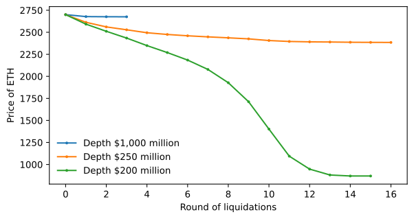

In a deep market, the first drop triggers a few liquidations, their sales barely move the price, and the cascade stops after a handful of rounds. As the market gets thinner, each round of sales pushes the price into the next group of liquidation prices, and the final fall is a multiple of the first. Below some depth the cascade runs away. In the thinnest market here, a first drop of 10% ends as a fall of about 70%: each round’s sales push the price into a denser part of the distribution of liquidation prices, the same loans are liquidated again and again, and some end with debt but no collateral, which is bad debt for the lenders.

The thinnest case also shows a feature of the rules. A liquidation repays debt and takes collateral worth 5% more. Repaying one dollar of debt removes 1.05 dollars of collateral, which counted 0.80 × 1.05 = 0.84 dollars toward the health factor. So for a loan whose health factor is already below 0.84, a liquidation leaves it less healthy than before, and it is liquidated again in the next round.

How the size of the first drop matters

In a market of 500 million dollars, first drops of different sizes:

rows = []
for drop in [0.05, 0.10, 0.15, 0.20]:
    r = cascade(500e6, drop)
    rows.append({"first drop": -drop, "final change in price": r["final_price"] / P0 - 1,
                 "rounds": r["rounds"], "liquidated ($ millions)": r["liquidated"] / 1e6,
                 "bad debt ($ millions)": r["bad_debt"] / 1e6})
pd.DataFrame(rows).set_index("first drop").style.format(
    {"final change in price": "{:+.1%}", "liquidated ($ millions)": "{:.1f}",
     "bad debt ($ millions)": "{:.1f}"}).format_index("{:+.0%}")

	final change in price	rounds	liquidated ($ millions)	bad debt ($ millions)
first drop
-5%	-5.1%	1	0.1	0.0
-10%	-12.2%	5	2.9	0.0
-15%	-20.5%	8	7.7	0.0
-20%	-31.3%	18	16.7	0.1

A small drop triggers almost nothing, because in our simulation no borrower started with a health factor below 1.05, so no loan becomes liquidatable until the price has fallen by about 5%. With more borrowers close to the limit, even a small drop would set off liquidations. Larger drops reach the dense part of the distribution, and the amplification grows: the cascade adds more to a large drop than to a small one.

What the simulation leaves out

Real markets are not a single pool. When liquidations push the price down on one exchange, arbitrageurs buy there and sell elsewhere, bringing in liquidity from the whole market, so the depth that matters is everything that can be traded within minutes. But that depth is not fixed: in a crash, market makers pull back and depth shrinks exactly when it is needed. Borrowers also react, adding collateral or repaying debt when the price falls, and protocols set thresholds, bonuses and borrowing caps with cascades like these in mind.

Try it

1. Raise the liquidation bonus to 10%, or let liquidators repay the whole debt at once (a close factor of 1). How do the cascades change?
2. Make borrowers more cautious: draw the starting health factors between 1.3 and 2.5. At what depth does the cascade in a 10% drop stop being much larger than the first drop?
3. Suppose the protocol’s oracle used the average price over the last few rounds instead of the current pool price. Modify cascade to do this. Does a delayed oracle make cascades smaller, and what new risk does it create?