from pathlib import Path

import matplotlib.pyplot as plt
import numpy as np
import pandas as pd
import requests
import yfinance as yf

DATA = Path("../_data") if Path("../_data").exists() else Path("data")
rng = np.random.default_rng(0)Trading Against an Automated Market Maker
This notebook builds a constant-product pool in a few lines of code, simulates arbitrageurs trading against it as the price of ETH moves, and checks that the liquidity providers’ loss matches the formula \sigma^2/8 of Milionis et al. (2022). It then turns to a real pool, Uniswap’s USDC-WETH pool on Ethereum, and asks whether its fees have paid for that loss. The notes on automated market makers explain the background.
Milionis, Jason, Ciamac C. Moallemi, Tim Roughgarden, and Anthony Lee Zhang. 2022. Automated Market Making and Loss-Versus-Rebalancing. https://arxiv.org/abs/2208.06046.
Packages
A pool in code
A pool is just two numbers, its reserves of ETH and USDC. Buying ETH from it means taking ETH out and putting in enough USDC to keep the product of the reserves unchanged. The fee, 0.30% in Uniswap’s original pools, is charged on the USDC paid in and stays in the pool.
def buy_eth(pool, eth_out, fee=0.003):
    """Buy eth_out ETH from the pool; return the USDC paid and the new pool."""
    eth, usdc = pool
    k = eth * usdc
    usdc_in = (k / (eth - eth_out) - usdc) / (1 - fee)
    return usdc_in, (eth - eth_out, usdc + usdc_in)

pool = (1_000.0, 3_000_000.0)       # 1,000 ETH and 3 million USDC: a price of 3,000
for size in [1, 10, 100, 300]:
    paid, _ = buy_eth(pool, size)
    print(f"buy {size:>3} ETH: pay {paid:12,.0f} USDC, average price {paid / size:8,.0f}")
buy 1 ETH: pay 3,012 USDC, average price 3,012
buy 10 ETH: pay 30,394 USDC, average price 3,039
buy 100 ETH: pay 334,336 USDC, average price 3,343
buy 300 ETH: pay 1,289,583 USDC, average price 4,299The bigger the trade relative to the pool, the more the average price exceeds the pool’s price of 3,000. This is the price impact of the constant-product rule.
Arbitrage against a moving price
Now let the market price of ETH move, and let an arbitrageur trade with the pool at every step until the pool’s price equals the market price. With no fee, the pool’s reserves after the trade are x = \sqrt{k/P} and y = \sqrt{kP}, so we can jump straight to them.
At each step, compare the pool with a portfolio that started the step with the same reserves and simply held them. The difference is what the arbitrageur took from the pool at that step: the pool sold ETH just after it became more valuable, or bought ETH just after it became less valuable. Summed over time, this is the loss versus rebalancing (LVR).
def simulate_lvr(sigma_annual, days=365, steps_per_day=24, paths=200):
    """Simulate ETH prices and an arbitraged constant-product pool.
    Returns cumulative LVR as a fraction of pool value, one column per path."""
    dt = 1 / (365 * steps_per_day)
    n = days * steps_per_day
    shocks = rng.standard_normal((n, paths))
    log_p = np.cumsum(-0.5 * sigma_annual**2 * dt + sigma_annual * np.sqrt(dt) * shocks, axis=0)
    price = 3_000 * np.exp(np.vstack([np.zeros(paths), log_p]))

    k = 1_000.0 * 3_000_000.0
    eth, usdc = np.sqrt(k / price), np.sqrt(k * price)   # reserves after arbitrage
    value = 2 * np.sqrt(k * price)                        # pool value
    held = eth[:-1] * price[1:] + usdc[:-1]               # last reserves, at the new price
    loss = (held - value[1:]) / value[1:]                 # this step's LVR, as a fraction
    return pd.DataFrame(np.cumsum(loss, axis=0),
                        index=np.arange(1, n + 1) / steps_per_day)

sigma = 0.80
lvr = simulate_lvr(sigma)
print(f"Average LVR after one year: {lvr.iloc[-1].mean():.2%} of the pool")
print(f"Formula sigma^2 / 8:        {sigma**2 / 8:.2%}")
Average LVR after one year: 8.00% of the pool
Formula sigma^2 / 8: 8.00%fig, ax = plt.subplots(figsize=(7, 3.5))
ax.plot(lvr.index, 100 * lvr.iloc[:, :50], color="0.85", lw=0.5)
ax.plot(lvr.index, 100 * lvr.mean(axis=1), lw=2, label="Average over 200 paths")
ax.plot(lvr.index, 100 * sigma**2 / 8 * lvr.index / 365, "--", label=r"$\sigma^2 t / 8$")
ax.set_xlabel("Days")
ax.set_ylabel("Cumulative LVR (% of pool)")
ax.legend(frameon=False)
plt.show()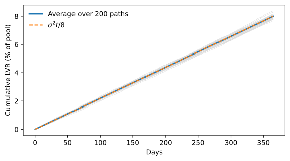
The loss accumulates steadily along every path, whether the price ends up higher or lower, and on average it follows \sigma^2 t/8. This is the point of the measure: it does not depend on where the price ends, only on how much it moves along the way.
Two assumptions make the formula exact: arbitrage happens continuously, and it is free. With a fee, arbitrageurs trade only when the gap between the pool’s price and the market price is larger than the fee, so the pool loses somewhat less. Try it with fees in the exercises.
A real pool: Uniswap v2 USDC-WETH
In a Uniswap v2 pool every liquidity provider holds the full constant-product curve, so every dollar in the pool earns the same fees and suffers the same loss. That makes it the right pool to test the formula. DefiLlama publishes its daily size and fee yield, free and without an account.
file = DATA / "defillama_univ2_usdc_weth.parquet"
if not file.exists():
    url = "https://yields.llama.fi/chart/702fff16-4bfa-4c1f-8c02-e0ea0f5ecde6"
    rows = requests.get(url, headers={"User-Agent": "FIN 4506 course notebook"},
                        timeout=60).json()["data"]
    DATA.mkdir(exist_ok=True)
    pd.DataFrame(rows).to_parquet(file)
uni = pd.read_parquet(file)
uni.index = pd.to_datetime(uni["timestamp"]).dt.tz_localize(None).dt.normalize()
uni = uni[["tvlUsd", "apyBase"]].rename(columns={"tvlUsd": "size", "apyBase": "fee_apy"})
uni.tail()| size | fee_apy | |
|---|---|---|
| timestamp | ||
| 2026-11-07 | 19187449 | 0.45875 |
| 2026-11-08 | 19155529 | 0.29557 |
| 2026-11-09 | 18742270 | 4.71087 |
| 2026-11-10 | 18361831 | 4.66010 |
| 2026-11-11 | 18459970 | 2.62523 |
fee_apy is the fee income of the past day as an annual percentage of the pool’s size. Dividing by 365 gives the day’s fees as a fraction of the pool. For the loss, we apply the formula day by day with that day’s squared return of ETH, from Yahoo Finance: r_t^2/8.
eth = yf.download("ETH-USD", start="2022-03-01", auto_adjust=True, progress=False)["Close"].squeeze()
daily = uni.join(np.log(eth).diff().rename("r")).dropna()
daily["fees"] = daily["fee_apy"] / 100 / 365
daily["lvr"] = daily["r"] ** 2 / 8

yearly = daily.resample("YE").agg({"fees": "sum", "lvr": "sum", "size": "mean"})
yearly["days"] = daily["fees"].resample("YE").count()
yearly.index = yearly.index.year.rename("year")
yearly.assign(fees=100 * yearly["fees"], lvr=100 * yearly["lvr"],
              size=yearly["size"] / 1e6).round(1).rename(columns={
    "fees": "fees (% of pool)", "lvr": "LVR (% of pool)", "size": "average size ($ millions)",
"days": "days with data"})| fees (% of pool) | LVR (% of pool) | average size ($ millions) | days with data | |
|---|---|---|---|---|
| year | ||||
| 2022 | 10.3 | 7.6 | 131.0 | 277 |
| 2023 | 5.7 | 2.4 | 66.4 | 320 |
| 2024 | 9.5 | 5.1 | 91.6 | 356 |
| 2025 | 9.2 | 6.8 | 31.4 | 359 |
| 2026 | 4.4 | 4.0 | 19.1 | 315 |
fig, (ax1, ax2) = plt.subplots(2, 1, figsize=(8, 5), sharex=True,
                               gridspec_kw={"height_ratios": [3, 2]})
ax1.plot(100 * daily["fees"].cumsum(), label="Fees earned")
ax1.plot(100 * daily["lvr"].cumsum(), label=r"Loss to arbitrageurs, $r_t^2/8$")
ax1.set_ylabel("Cumulative (% of pool)")
ax1.legend(frameon=False)
ax2.plot(daily["size"] / 1e6)
ax2.set_ylabel("Pool size ($ millions)")
plt.show()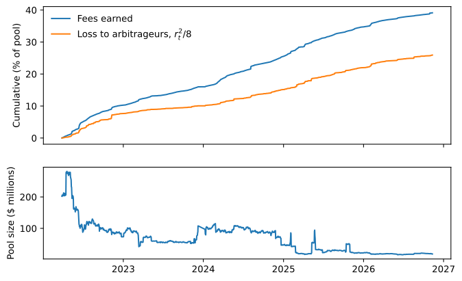
Two things to know about the table. The first and last years are partial: the data start on March 27, 2022, and end in November 2026. And DefiLlama’s series misses some days, 31 of them around the turn of 2024; on missing days neither fees nor losses are counted, so those years’ sums understate both.
Fees have exceeded the loss to arbitrageurs in every year, by a margin that was thin in volatile years and close to zero in 2026. Meanwhile the pool has shrunk. The table cannot tell us why. Lehar and Parlour (2025) show the logic of an equilibrium in which the pool’s size adjusts until liquidity providers’ fees just compensate them for being picked off by arbitrageurs. But compensation here must also cover the alternative uses of the capital, and a margin of a few percentage points over the loss is not much when Treasury bills pay 4% to 5%. Liquidity may also have moved to Uniswap’s later versions. Telling these explanations apart would take more data than this pool provides.
Lehar, Alfred, and Christine Parlour. 2025. “Decentralized Exchange: The Uniswap Automated Market Maker.” Journal of Finance 80 (1): 321–74. https://doi.org/10.1111/jofi.13405.
Try it
- Add a fee to the simulation: at each step, let the arbitrageur trade only when the pool’s price is more than 0.30% away from the market price, and then only enough to bring the pool’s price back to the edge of that band. The fee the arbitrageur pays stays in the pool. How much smaller is the pool’s net loss?
- Run the simulation with an annual volatility of 46% and of 108%, the lowest and highest yearly volatility of ETH since 2018. How does the loss scale?
- A liquidity provider deposited in this pool at the start of 2024. Using the daily data, what were their fees minus their loss by the end of 2025?